Joint and Conditional Entropy

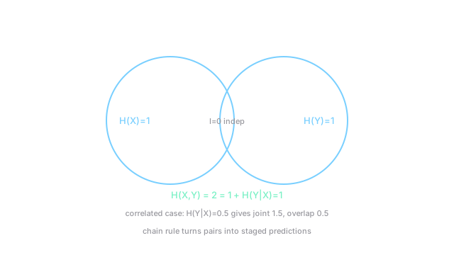
Pairs carry joint surprise; knowing one variable discounts the other. The chain rule splits the pair into staged, additive predictions.

Two independent fair coins show joint entropy 2 with conditional 1 each, chaining exactly as H(X) plus H(Y|X)

Why Does This Exist?

Features arrive in bundles: pixels, tokens, sensors. Pricing the bundle's surprise as the sum of singles overcounts whenever variables correlate, and undercounts nothing ever. Compression, feature selection, and sequential prediction all need the pair price and the discount-for-knowing.

Definitions: $H(X,Y) = -\\sum p(x,y)\\log p(x,y)$ and $H(Y\\mid X) = H(X,Y) - H(X)$ , averaging $H(Y\\mid X=x)$ over $x$ . Chain: $H(X,Y) = H(X) + H(Y\\mid X)$ . It extends entropy to pairs and feeds mutual information as the overlap.

The one idea you need first

Entropy averages $-\\log p$ : fair coin $-(0.5\\log_2 0.5 + 0.5\\log_2 0.5) = 1$ bit. Joint entropy runs the same average over pairs; conditional subtracts what $X$ already told you.

Think of It Like This

Two weather reporters

Two reporters cover neighboring towns. Reading both fresh takes two minutes (joint). Reading the second after the first takes less: shared weather isold news (conditional discount).

Independent towns: no discount. Identical towns: second report free. Where it stops: reporters editorialize, adding noise. Conditional entropy assumes the true joint, not two biased retellings.

How It Actually Works

Chain generalizes: $H(X_1,\\ldots,X_n) = \\sum_i H(X_i \\mid X_{<i})$ , the compression order matters only for the splits, never the total. Conditioning reduces entropy: $H(Y\\mid X) \\leq H(Y)$ , equality for independence. MI is the discount: $I(X;Y) = H(Y) - H(Y\\mid X) = H(X) + H(Y) - H(X,Y)$ . Estimation from counts needs smoothing; plug-in underestimates with few samples (Miller-Madow corrects $+ (m-1)/2n$ in nats).

Worked example

Two independent fair coins: 4 pairs at $1/4$ each, $H(X,Y) = -4(0.25\\log_2 0.25) = 2$ bits. $H(X) = 1$ , $H(Y\\mid X) = 1$ , chain $1 + 1 = 2$ . Correlate: $P(00) = P(11) = 0.4$ , $P(01) = P(10) = 0.1$ . Margins stay fair (1 bit each), joint $= -2(0.4\\log_2 0.4) - 2(0.1\\log_2 0.1) = 2(0.5288) + 2(0.3322) = 1.722$ bits. Conditional $0.722$ , MI $0.278$ : correlation donated 0.278 bits of discount.

Code

1import numpy as np2
3p = np.array([0.4, 0.1, 0.1, 0.4])  # 00,01,10,114h_joint = float(-(p * np.log2(p)).sum())5print(round(h_joint, 3))  # -> 1.7226print(round(h_joint - 1.0, 3))  # -> 0.722 conditional

Joint 1.722 minus 1 bit margin leaves 0.722 conditional. Same margins, dependence moves the total.

Watch Out For

Summing marginal entropies for correlated features

Adding per-feature entropies double-counts shared bits: joint can be far below the sum (1.722 vs 2.0 above). Feature-selection budgets built on sums overbuy capacity.

Price bundles jointly or subtract MI. If features correlate above 0.5, the sum is fiction.

Trusting plug-in entropy on small samples

Few samples make rare pairs invisible, so plug-in $\\hat H$ runs low by roughly $(m-1)/2n$ nats. Lane: 100 samples over 64 pairs biases down ~0.3 nats (~0.45 bits).

Smooth, use Miller-Madow or NSB estimators, or collect more. If unseen pairs abound, the estimate is a floor.

The Quick Version

Joint entropy prices pairs; conditional prices the remainder after knowing one.
Chain: $H(X,Y) = H(X) + H(Y\\mid X)$ ; $n$ -way chains telescope the same way.
Independent fair coins total 2 bits; the correlated example totals 1.722 with MI 0.278.
Conditioning never increases entropy; independence holds equality.
Never sum margins for correlated bundles; subtract the overlap.
Smooth small-sample estimates or quote them as floors.