Kalman Filters

Tracking a hidden number by blending what motion predicts with what the sensor says, trusting each exactly as much as its uncertainty earns.

A prior estimate of 2.0 with wide uncertainty and a sensor reading of 2.5 blend through a gain of 0.69 into a fused estimate of 2.34

Why Does This Exist?

A robot never sees its position. It sees wheel odometry that drifts and GPS fixes that jitter, and it must turn both into one best guess that updates as it moves. Averaging them with fixed weights fails the moment conditions change: in a tunnel the GPS deserves no vote, on open road it deserves a large one. What is needed is a blend whose weights breathe with the uncertainties.

The Kalman filter is that blend for the linear-Gaussian world, and it is optimal there: no other estimator has smaller mean squared error. Motion and sensing are both linear with additive Gaussian noise, the belief stays Gaussian forever, and each step is two closed-form moves: predict forward through motion, then correct with the observation. When the world goes nonlinear or the noise goes multimodal, this page is still the right prerequisite, because every successor (particle filters, extended and unscented variants) is best understood as what you reach for when one Kalman assumption breaks. The Gaussian machinery underneath is in multivariate Gaussians, and the time structure is a Markov chain.

The one idea you need first

A Gaussian stays Gaussian through linear maps and conditioning. So if the state starts Gaussian and every transition and observation is linear plus Gaussian noise, the posterior after any number of steps is still Gaussian, fully described by a mean and a covariance. The filter just tracks those two.

Think of It Like This

A navigator blending dead reckoning with landmarks

A sailor dead-reckons: from the last fix, speed and heading say where you should be, but errors accumulate with every mile. Then a lighthouse bearing arrives: it says where you are, but the bearing itself has error.

The sailor does not pick one. On a foggy night with a sharp log, the reckoning gets most of the vote. After a long run with no fixes followed by a crisp noon sight, the sight dominates. The blend ratio is set by the two uncertainties, and after fusing, the sailor is more confident than either source alone.

Where the analogy stops: the filter also tracks how that confidence evolves, growing it during blind motion and shrinking it at each sighting, by exact arithmetic rather than judgement.

How It Actually Works

State $x_t$ evolves and observation $y_t$ arrives by

x_t = F x_{t-1} + w_t, \qquad y_t = H x_t + v_t

where $F$ is the motion matrix, $H$ maps state to sensor, $w_t$ has covariance $Q$ (motion noise), and $v_t$ has covariance $R$ (sensor noise). The belief is $\hat{x}$ (mean) with $P$ (covariance).

Predict. Push through motion: $\hat{x}_{t\mid t-1} = F \hat{x}_{t-1}$ , $P_{t\mid t-1} = F P_{t-1} F^\top + Q$ . Uncertainty always grows here: motion adds $Q$ .

Update. Compute the Kalman gain $K = P_{t\mid t-1} H^\top (H P_{t\mid t-1} H^\top + R)^{-1}$ , then $\hat{x}_t = \hat{x}_{t\mid t-1} + K(y_t - H\hat{x}_{t\mid t-1})$ and $P_t = (I - KH)P_{t\mid t-1}$ . In plain words: $K$ is prediction-uncertainty divided by total uncertainty, so a precise sensor ( $R$ small) pulls hard toward the reading and a vague one barely nudges.

Worked example

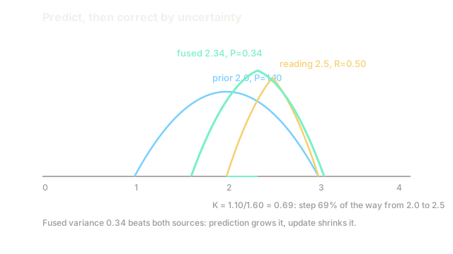
Scalar tracking, static state ( $F = 1$ , $H = 1$ ). Prior $\hat{x} = 2.0$ with $P = 1.0$ , motion noise $Q = 0.10$ , reading $y = 2.5$ with $R = 0.50$ .

Predict: $\hat{x} = 2.0$ unchanged, $P = 1.0 + 0.10 = 1.10$ .

Gain: $K = 1.10 / (1.10 + 0.50) = 1.10/1.60 = 0.6875$ . The sensor earns a 69 percent vote because $0.50$ against $1.10$ is the more precise of the two.

Update: $\hat{x} = 2.0 + 0.6875 \times (2.5 - 2.0) = 2.0 + 0.34375 = 2.34375$ . Covariance: $P = (1 - 0.6875) \times 1.10 = 0.34375$ , below both $1.10$ and $0.50$ : fusing beats either source alone.

Watch Out For

Running a linear filter on a nonlinear world

Apply the standard equations to a radar that measures range and bearing, or a pendulum near horizontal, and the linearization point drifts while $F$ and $H$ pretend the world is flat. The covariance shrinks exactly as if the linear model were true, so the filter grows confident around a wrong estimate and starts rejecting the very readings that could save it.

Symptom: normalized residuals (innovations divided by their predicted spread) drift far above 1 while the reported $P$ stays small. Fix: use an extended or unscented variant for mild nonlinearity, and move to particle filters when posteriors go multimodal.

Letting the covariance go asymmetric or negative

$P$ must stay symmetric positive definite, but the update $(I - KH)P$ subtracts two nearly equal matrices in finite precision. After thousands of steps $P$ can develop a tiny asymmetry or a negative eigenvalue, and then the next gain is garbage: uncertainty that should shrink explodes instead.

Symptom: filter diverges after long healthy runs, with $P$ showing asymmetry beyond $10^{-12}$ or negative diagonal entries. Fix: use the Joseph form $P = (I-KH)P(I-KH)^\top + KRK^\top$ , symmetrize each step with $(P + P^\top)/2$ , and never invert the innovation covariance without checking its conditioning.

The Quick Version

A Kalman filter tracks a Gaussian belief through linear motion and linear sensing, alternating predict and update.
The Kalman gain weights the reading by prediction-uncertainty over total uncertainty.
In the worked pass, prior 2.0 and reading 2.5 fuse to 2.34 with variance 0.34, better than either source.
Prediction always grows uncertainty; update always shrinks it.
Nonlinear or non-Gaussian worlds need extended, unscented, or particle variants.
Guard the covariance update numerically or long runs diverge.