Sequential Monte Carlo Particle Filters

Tracking a moving target with a cloud of guesses. Thousands of weighted particles chase the posterior through time, cloning the good ones.

Five particles spread by motion noise get reweighted by the new observation, then resampling clones the two best and drops the two worst

Why Does This Exist?

Some posteriors move. A robot localizes, a phone tracks a voice, a fund estimates volatility: each new observation should update the belief about a hidden state that itself evolves. When the motion and the sensors are linear and Gaussian, the Kalman filter answers in closed form. When they are nonlinear or the noise is multimodal, no closed form exists, and the particle filter is the workhorse: it represents the filtering distribution with a cloud of weighted samples propagated through time.

Each step has three moves: propose particles forward through the motion model, weight them by how well they explain the new observation, and resample to clone the winners. That last step is the difference between a filter and a slow collapse, and it is where beginners go wrong.

The one idea you need first

Importance sampling estimates expectations under $p$ with samples from $q$ by weighting each sample with $p/q$ . A particle filter applies this sequentially: the proposal is the motion model and the weight update is the observation likelihood. The static version is covered alongside Monte Carlo methods.

Think of It Like This

A search party with radios

A lost hiker moves through hills while the search team holds five guesses of the position. Each hour, every guess walks forward according to the hiker's habits (the motion model), spreading out. Then a helicopter reports a glimpse: guesses near the glimpse get high weight, far ones get near zero. Finally the team regroups: members holding bad guesses walk over to copy the good ones, so all five guesses cluster near the evidence before the next hour starts.

Without the regrouping step, after a few hours four of five guesses would be hopelessly lost and only one would carry all the weight: the team wasted. Resampling is the regroup. The price is milder: cloned guesses share ancestors, so diversity must come from the motion noise injected each round.

Where the analogy stops: real filters carry thousands of particles, not five, and the regroup uses a single systematic draw rather than a team decision.

How It Actually Works

State $x_t$ evolves by $p(x_t \mid x_{t-1})$ and observation $y_t$ arrives by $p(y_t \mid x_t)$ . Given particles $\{x_{t-1}^{(i)}, w_{t-1}^{(i)}\}$ , one filtering step is:

Propagate. Draw $x_t^{(i)} \sim p(x_t \mid x_{t-1}^{(i)})$ .
Weight. Set $\tilde{w}_t^{(i)} \propto w_{t-1}^{(i)} p(y_t \mid x_t^{(i)})$ , then normalize.
Resample (when needed). Draw $N$ new particles with probabilities $\tilde{w}_t^{(i)}$ and reset all weights to $1/N$ .

The filtered mean $\sum_i w_t^{(i)} x_t^{(i)}$ estimates the hidden state. Resample when the effective sample size $1/\sum_i (w_t^{(i)})^2$ falls below about $N/2$ ; resampling every step is simpler and fine for an introduction.

Worked example

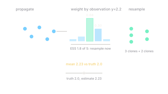
Five particles sit at $[1.0, 1.5, 2.0, 2.5, 3.0]$ with equal weights. Motion adds noise giving $[1.2, 1.4, 2.1, 2.6, 3.2]$ . Truth is $x = 2.0$ and the sensor reports $y = 2.2$ with Gaussian noise of standard deviation $0.3$ . Likelihood weights are proportional to $\exp(-(x - 2.2)^2 / 0.18)$ :

$x = 1.2$ : $\exp(-1/0.18) \approx 0.004$
$x = 1.4$ : $\exp(-0.64/0.18) \approx 0.028$
$x = 2.1$ : $\exp(-0.01/0.18) \approx 0.946$
$x = 2.6$ : $\exp(-0.16/0.18) \approx 0.411$
$x = 3.2$ : $\exp(-1/0.18) \approx 0.004$

Normalized: $[0.003, 0.020, 0.679, 0.295, 0.003]$ . The weighted mean is $1.2(0.003) + 1.4(0.020) + 2.1(0.679) + 2.6(0.295) + 3.2(0.003) \approx 2.23$ . Resampling five draws from these weights yields, for one typical outcome, particles $[2.1, 2.1, 2.1, 2.6, 2.6]$ : the two best ancestors survive, the two worst vanish, and the equal-weight mean $2.30$ sits $0.30$ above truth $2.0$ before the next motion step corrects it. Effective sample size is $1/(0.003^2 + 0.020^2 + 0.679^2 + 0.295^2 + 0.003^2) \approx 1.82$ : resampling was overdue, which is the normal state of affairs.

Code

The worked pass in code: propagate, weight by the Gaussian likelihood, report the effective sample size.

1import numpy as np2
3rng = np.random.default_rng(9)4parts = np.array([1.0, 1.5, 2.0, 2.5, 3.0])  # particles5parts = parts + rng.normal(0, 0.2, size=5)  # motion noise6w = np.exp(-0.5 * ((parts - 2.2) / 0.3) ** 2)  # observation y=2.27w = w / w.sum()  # normalize8print(np.round(w, 3))  # -> mass on the two nearest9print(round(float((w**2).sum() ** -1), 2))  # -> effective sample size

Weights concentrate on the particles nearest 2.2 and the effective size prints well below 5, signalling resampling. Add parts = rng.choice(parts, size=5, p=w) to resample and watch the losers disappear.

Watch Out For

Skipping resampling until one particle owns everything

Without resampling, weights compound multiplicatively and within a dozen steps a single particle carries 99.9 percent of the mass: thousands of likelihood evaluations wasted on ghosts. Monitor the effective sample size every step and resample below $N/2$ . This degeneracy is silent, the mean still prints, so the monitor must be code, not eyeballing.

Resampling noise swamping a small particle set

With only dozens of particles, resampling variance itself dominates: good ancestors die by bad luck and the filter jitters. Use systematic resampling (one uniform draw, evenly spaced thresholds) instead of multinomial draws, and scale $N$ with state dimension. A 10-dimensional state with 100 particles is hope, not filtering.

The Quick Version

A particle filter tracks a moving posterior with weighted samples through propagate, weight, resample.
Weights are the observation likelihood; the weighted mean estimates the hidden state.
In the worked pass the two particles nearest the observation take 97 percent of the mass.
Effective sample size near 1.8 out of 5 means resample now, not later.
No resampling gives degeneracy: one particle owns everything within a dozen steps.
Linear Gaussian cases deserve a Kalman filter instead; particles earn their cost on nonlinear ones.