Kronecker Product

A product that builds big structured matrices out of small ones, block by block. It is how independent systems combine into one joint system.

Each entry of the left matrix scales a full copy of the right matrix, so a 2 by 2 with a 2 by 2 tiles into a 4 by 4 of blocks

Why Does This Exist?

Two independent linear systems combine into one joint system all the time: two sensors with their own covariances, a grid that is a product of one-dimensional grids, a layer acting on rows and another on columns. Writing the joint operator out entry by entry is miserable. The Kronecker product $A \otimes B$ builds it in one move: every entry $a_{ij}$ scales a full copy of $B$ into a block.

Its superpower is the vec trick: $\mathrm{vec}(AXB) = (B^T \otimes A)\,\mathrm{vec}(X)$ . A matrix equation in three unknowns-shaped pieces becomes one ordinary linear system, which is how Lyapunov equations, Gaussian process grid covariances and second-order optimiser approximations get solved rather than admired.

The one idea you need first

Vectorisation $\mathrm{vec}(X)$ stacks a matrix's columns into one long vector. Block matrices multiply block by block. With those two pictures the definition below reads as tiling, not algebra.

Think of It Like This

A mosaic ordered from a catalogue

A catalogue sells two tile sheets: sheet A holds 2 by 2 large pattern tiles, sheet B holds 2 by 2 small detail tiles. Ordering "A in B" means: take the layout of A, and replace every single large tile with a complete copy of sheet B, scaled by that tile's shade.

The result is 4 by 4: the coarse structure comes from A, the fine structure inside each block comes from B. Swapping the order ("B in A") gives a different mosaic, because which pattern is coarse and which is fine has flipped. Non-commutativity you can see.

The analogy stops at sizes: real Kronecker products blow up multiplicatively (100 by 100 with 100 by 100 is 10,000 by 10,000), while mosaics stay on the wall. Never form one you only need to multiply through.

How It Actually Works

For $A$ of size $m \times n$ and $B$ of size $p \times q$ , $A \otimes B$ is $mp \times nq$ , built block by block:

A \otimes B = \begin{bmatrix} a_{11}B & \cdots & a_{1n}B \\ \vdots & \ddots & \vdots \\ a_{m1}B & \cdots & a_{mn}B \end{bmatrix}

Three properties do the heavy lifting:

Mixed product: $(A \otimes B)(C \otimes D) = (AC) \otimes (BD)$ . Factored computation stays factored.
Vec trick: $\mathrm{vec}(AXB) = (B^T \otimes A)\,\mathrm{vec}(X)$ . Matrix equations become linear systems.
Spectrum: eigenvalues multiply pairwise ( $\lambda_i \mu_j$ ), so determinants and inverses factor too: $(A \otimes B)^{-1} = A^{-1} \otimes B^{-1}$ .

Worked example

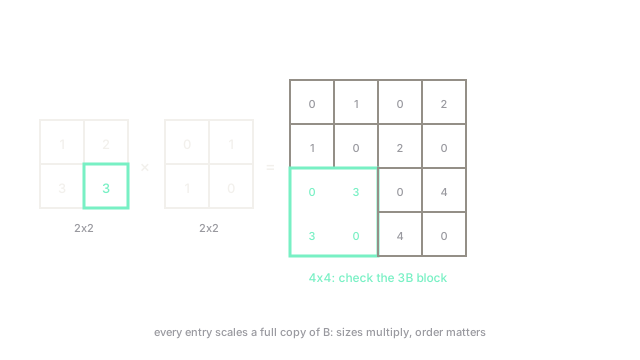
Build $\begin{bmatrix} 1 & 2 \\ 3 & 4 \end{bmatrix} \otimes \begin{bmatrix} 0 & 1 \\ 1 & 0 \end{bmatrix}$ . Each entry scales a full copy of the right matrix:

\begin{bmatrix} 1 \cdot B & 2 \cdot B \\ 3 \cdot B & 4 \cdot B \end{bmatrix} = \begin{bmatrix} 0 & 1 & 0 & 2 \\ 1 & 0 & 2 & 0 \\ 0 & 3 & 0 & 4 \\ 3 & 0 & 4 & 0 \end{bmatrix}

Check one block: bottom-left is $3B = [[0, 3], [3, 0]]$ , sitting in rows 3 to 4, columns 1 to 2. The result is 4 by 4 from two 2 by 2 inputs, and its eigenvalues are the pairwise products of $\{5, -1\}$ -ish spectra. Tiling, exactly as advertised.

Code

The point is the check: build the product and verify the mixed-product property numerically.

1import numpy as np2
3
4A = np.array([[1, 2], [3, 4]])5B = np.array([[0, 1], [1, 0]])6K = np.kron(A, B)7print(K.tolist())  # -> [[0, 1, 0, 2], [1, 0, 2, 0], [0, 3, 0, 4], [3, 0, 4, 0]]8C = np.array([[1, 0], [0, 1]])9print(np.allclose(np.kron(A, B) @ np.kron(C, B), np.kron(A @ C, B @ B)))  # -> True

Watch Out For

Assuming the product commutes

$A \otimes B \ne B \otimes A$ in general: the block structures differ (they are permutation-similar, not equal). Code that swaps the order "for efficiency" scrambles which subsystem is which, and square test cases can pass while rectangular ones fail. Keep a fixed subsystem order across the whole pipeline.

Forming a product you only multiply through

$A \otimes B$ for 1,000-dimensional factors is a million-by-million matrix you cannot store, but $(A \otimes B)x$ computes through the factors in $O(n^3)$ instead of $O(n^4)$ via the vec trick. Form the product only for tiny teaching examples; in production, multiply through the structure.

The Quick Version

$A \otimes B$ replaces every entry $a_{ij}$ with the block $a_{ij}B$ : tiling, block by block.
The 2-by-2 example tiles into the 4-by-4 shown above; check the $3B$ block to believe it.
Mixed product keeps factored computation factored; the vec trick linearises $AXB$ .
Eigenvalues multiply pairwise, and inverses factor across the product.
Never form huge Kronecker matrices explicitly; multiply through the factors instead.