Lagrange Multipliers

The best point on a boundary is where your goal's contours just touch it. The multiplier measures how much loosening the boundary would be worth.

The hyperbola x times y equals 25 just touches the line x plus y equals 10 at (5, 5), where the two gradients line up and the multiplier reads 5

Why Does This Exist?

Unconstrained optimization is the easy case, and it is rarely the real one. Budgets are fixed, margins must hold, probabilities must sum to one, and weight norms get capped. The moment a rule you cannot break enters, setting the gradient to zero stops working, because the unconstrained peak usually sits outside the allowed region.

Lagrange multipliers handle equality constraints with one geometric insight: at the best allowed point, you cannot improve without leaving the region, which means the goal's contours run tangent to the boundary there. That tangency becomes a system of equations you can solve. It is the prerequisite for the duality theory in constrained optimisation and duality and for inequality constraints via KKT conditions, and its gradients-alignment picture is pure gradients geometry.

The one idea you need first

The gradient points in the steepest-ascent direction, perpendicular to the level curves. If the best feasible point were not a tangency, the goal's contour would cut across the constraint, and walking along the constraint in the cutting direction would improve the objective while staying feasible. So at an optimum the contour cannot cut; it must touch, and touching curves share parallel gradients.

Think of It Like This

The biggest field from a fixed length of fence

You own 100 metres of fence and want the largest rectangular field. Any rectangle using less fence can be stretched, so the winner uses it all. Now consider improving a candidate: widening forces shortening, and the trade gains area exactly when the marginal gain of width beats the marginal loss of height.

You stop when no trade helps, when widening gains exactly what shortening loses. Geometrically the area contours just touch the fence line. And the multiplier answers the follow-up question: what is one more metre of fence worth? That price interpretation survives into economics, where multipliers are called shadow prices, and into ML, where a multiplier on a fairness constraint prices fairness in accuracy.

The analogy stops at equality. Real fences also allow using less, an inequality, and handling slack needs the KKT extension rather than this page's method.

How It Actually Works

To maximize or minimize $f(x)$ subject to $g(x) = 0$ , build the Lagrangian:

\mathcal{L}(x, \lambda) = f(x) - \lambda\, g(x)

In plain words: the objective minus one penalty term per constraint, where each multiplier $\lambda$ is an unknown price for violating its constraint. Then solve the stationary system: $\nabla_x \mathcal{L} = 0$ alongside $g(x) = 0$ . The first block says $\nabla f = \lambda \nabla g$ , the gradients are parallel, which is the tangency. The second block says the point is feasible. With $n$ variables and $m$ constraints that is $n + m$ equations for $n + m$ unknowns.

Read the multiplier after solving: $\lambda$ is the rate at which the optimal value improves per unit of loosened constraint. If $\lambda = 5$ , one more unit of budget buys 5 units of objective. That reading is what makes the answer interpretable rather than mechanical.

Worked example

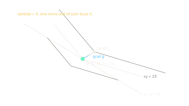
Maximize $f(x, y) = xy$ subject to $x + y = 10$ , with $x, y \geq 0$ .

The Lagrangian is $\mathcal{L} = xy - \lambda(x + y - 10)$ . Stationarity gives $y - \lambda = 0$ and $x - \lambda = 0$ , so $x = y = \lambda$ . Feasibility gives $2\lambda = 10$ , so $\lambda = 5$ and the candidate is $(5, 5)$ with value $25$ .

Confirm it is the maximum, not a minimum or saddle: the feasible segment runs from $(0, 10)$ to $(10, 0)$ , where $f = 0$ at both ends, and $25 > 0$ inside. So $(5, 5)$ wins. And the multiplier prices the constraint: raising the sum to $11$ gives $(5.5, 5.5)$ with value $30.25$ , an increase of $5.25$ for one unit, close to the predicted $5$ and exact in the limit.

Watch Out For

Solving the system and skipping the verification

Stationarity finds candidates, and constraints can hide minima, maxima, and saddles among them. The method never labels which is which. Always evaluate the objective at every candidate plus the feasible region's endpoints or boundary, as the worked example does with the zero-valued ends. An unverified candidate is a guess with algebra.

Applying equality machinery to inequalities

The tangency picture assumes the optimum sits on the constraint. With $x + y \leq 10$ the unconstrained peak of a concave objective may sit strictly inside, where the constraint is irrelevant and forcing tangency invents a wrong answer. Equality constraints use this page; inequalities need KKT conditions, which add the complementary-slackness switch that turns idle constraints off.

The Quick Version

Equality constraints are solved by tangency: at the optimum the objective contours touch the feasible region.
The Lagrangian subtracts one priced penalty per constraint, and stationarity plus feasibility give the candidates.
The multiplier is the shadow price: optimal value gained per unit of loosened constraint.
Maximizing xy on a sum of 10 picks (5, 5) with value 25 and multiplier 5.
Stationarity proposes; evaluating candidates and boundaries disposes.