Math

Gradients

A list of slopes, one per knob, that together point in the single direction where the error climbs fastest — so the opposite direction is where training goes.

$On a contour map of the loss, the gradient at a point is the arrow crossing the level curves at a right angle, pointing straight uphill; training steps the opposite way$

On a contour map of the loss, the gradient at a point is the arrow crossing the level curves at a right angle, pointing straight uphill; training steps the opposite way

Why Does This Exist?

Every trained model in production got there by asking one question, several million times: if I nudge this one number, does the error go up or down, and by how much? A model with 7 billion parameters asks it 7 billion times per step. The answer, collected into a single object, is the gradient.

Without it there is no training. You would be left guessing at parameter values, and the space is far too large to guess in — a network with only 100 parameters has more directions to try than there are atoms in your body. The gradient replaces search with a bearing: it tells you, from wherever you currently stand, exactly which way is downhill and how steep the slope is.

This page is about the object — what it is, what it points at, and what its size means. Gradient descent is the loop that repeatedly consumes it; backpropagation is the algorithm that computes it efficiently through a deep network. Both are far easier to follow once the object itself is clear, which is the job here.

The one idea you need first

A derivative is a rate of change. If a function $f$ takes one input and $f'(3) = 4$ , that means: standing at $x = 3$ , increasing $x$ by a tiny amount increases $f$ by about four times that amount. Steep positive slope.

A partial derivative is the same measurement when there is more than one input, taken while holding every other input still. Write it $\partial f / \partial x$ — "how much does $f$ change per unit of $x$ , with everything else frozen." That is the whole prerequisite. The full treatment is in derivatives and partial derivatives.

Think of It Like This

A hillside, and a compass that only points uphill

You are standing somewhere on a hillside in fog. You cannot see the valley, but you can feel the ground under your feet. Turn to face north: the ground rises steeply. Face east: it rises gently. Those two numbers — the north slope and the east slope — are your two partial derivatives.

Here is the part that makes the gradient useful rather than merely descriptive. Those two numbers, treated as a pair of coordinates, form an arrow. And that arrow points in the single steepest uphill direction available to you — not north, not east, but the exact compass bearing that climbs fastest. You did not have to try every direction to find it. Two measurements determined it.

Turn around and walk. That is training.

How It Actually Works

Take a loss $\mathcal{L}$ that depends on parameters $w_1, w_2, \ldots, w_n$ . The gradient is simply every partial derivative collected into one vector:

\nabla \mathcal{L} = \left[ \frac{\partial \mathcal{L}}{\partial w_1},\ \frac{\partial \mathcal{L}}{\partial w_2},\ \ldots,\ \frac{\partial \mathcal{L}}{\partial w_n} \right]

In plain words: one number per parameter, each saying how much the loss would rise if you increased that parameter alone. The symbol $\nabla$ is read "nabla" or "del". Shape matters and it is reassuringly simple — the gradient always has exactly the same shape as the thing you differentiated with respect to. A weight matrix of shape $200 \times 50$ has a gradient of shape $200 \times 50$ . If your shapes disagree, you have a bug, and that check catches a lot of them.

Why it points the steepest way

This is the property that earns the gradient its place, and it is worth seeing rather than accepting.

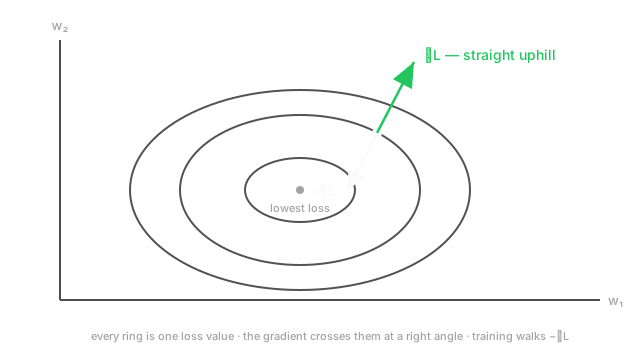
The rate of change as you move in some unit direction $u$ is the dot product $\nabla \mathcal{L} \cdot u$ . A dot product of two vectors is largest when they point the same way, so the direction that maximises your rate of climb is $u$ aligned with $\nabla \mathcal{L}$ itself. Every other direction gives you a smaller number — and directions at right angles to the gradient give you zero, which is exactly why the gradient crosses the contour lines of the loss at a right angle in the diagram above. Along a contour, the loss is not changing at all.

So the gradient points at steepest ascent. Training wants descent, which is why the update carries a minus sign, and why a stray sign error makes a model get reliably worse.

Two numbers, not one

The gradient carries a direction and a magnitude, and they mean different things:

The direction — which way to go. This is what the optimiser follows.
The magnitude $\lVert \nabla \mathcal{L} \rVert$ — how steep the slope is. This is a diagnostic, and the one practitioners actually watch. A magnitude collapsing toward zero means learning has stalled (vanishing gradients, or a genuine minimum). A magnitude exploding means the step about to be taken is enormous, which is what gradient clipping exists to cap. Measuring that length is what norms are for.

Worked example

Take $f(w_1, w_2) = w_1^2 + 3w_2^2$ and stand at the point $(2, 1)$ .

Differentiate each variable in turn, holding the other still. For $w_1$ , the $3w_2^2$ term is a constant and contributes nothing, so $\partial f / \partial w_1 = 2w_1$ . For $w_2$ , the $w_1^2$ term is the constant, so $\partial f / \partial w_2 = 6w_2$ . Substituting the point:

\nabla f(2, 1) = [\,2 \times 2,\ 6 \times 1\,] = [\,4,\ 6\,]

So the loss climbs fastest in the direction $[4, 6]$ — noticeably steeper in $w_2$ than in $w_1$ , even though we are further from the origin in $w_1$ . That asymmetry comes from the coefficient 3, and it is the reason this bowl's contours are stretched ellipses rather than circles.

Its magnitude is $\sqrt{4^2 + 6^2} = \sqrt{52} \approx 7.21$ . Training would step in the direction $[-4, -6]$ .

Show Me the Code

The point of this snippet is not the formula — it is the check. Comparing an analytic gradient against a finite-difference estimate is how you find out whether a hand-derived derivative is actually correct, and it is standard practice when implementing a custom layer or loss.

1import numpy as np2
3
4def f(w: np.ndarray) -> float:5    return float(w[0] ** 2 + 3 * w[1] ** 2)6
7
8def grad_analytic(w: np.ndarray) -> np.ndarray:9    return np.array([2 * w[0], 6 * w[1]])  # shape (2,) — same shape as w10
11
12def grad_numeric(w: np.ndarray, h: float = 1e-5) -> np.ndarray:13    out = np.zeros_like(w, dtype=float)14    for i in range(w.size):15        step = np.zeros_like(w, dtype=float)16        step[i] = h  # perturb one coordinate, hold the rest still17        out[i] = (f(w + step) - f(w - step)) / (2 * h)  # central difference18    return out19
20
21w = np.array([2.0, 1.0])22print(grad_analytic(w))                                  # -> [4. 6.]23print(np.allclose(grad_analytic(w), grad_numeric(w)))    # -> True

Both routes agree on $[4, 6]$ , which is the number the worked example derived by hand. The central difference is used rather than the one-sided $(f(w+h) - f(w))/h$ because it is accurate to $O(h^2)$ instead of $O(h)$ — a free improvement for the same amount of arithmetic.

Watch Out For

Shrinking h until the gradient check breaks

The obvious instinct when a gradient check nearly passes is to make $h$ smaller. Do that and the check gets worse, which sends people hunting for a bug that was never in their derivative.

The cause is catastrophic cancellation. $f(w+h)$ and $f(w-h)$ agree in their leading digits, and subtracting two nearly equal floating-point numbers throws those digits away — at float64 you have roughly 16 significant digits to spend, and a tiny $h$ spends nearly all of them before the division by $2h$ amplifies whatever noise is left. At $h = 10^{-12}$ the result is mostly garbage.

Truncation error falls as $h$ shrinks while round-off error grows, so the total is U-shaped. Sit near the bottom: $h \approx 10^{-5}$ for float64, and compare with a relative tolerance rather than an absolute one. Never gradient-check in float32.

Following the gradient instead of fleeing it

The gradient points uphill. Training goes downhill. So the update subtracts, and w += lr * grad instead of w -= lr * grad is a real bug that gets written regularly — most often when someone hand-rolls an optimiser, or flips the sign of a loss to turn a minimisation into a maximisation and forgets to flip the update too.

It does not crash. It does not warn. The loss simply climbs, smoothly and confidently, and it looks exactly like a learning rate that is too high. If your loss rises from the very first step and lowering the learning rate only makes it rise more slowly, check the sign before you touch anything else.

The Quick Version

A gradient is every partial derivative of a function, collected into one vector — one slope per parameter.
It always has the same shape as the parameters you differentiated with respect to. Mismatched shapes mean a bug.
Its direction is steepest ascent, so training subtracts it. That minus sign is not decoration.
It is perpendicular to the contour lines of the loss, because moving along a contour changes nothing.
Its magnitude is the steepness, and it is the number to watch: collapsing toward zero means stalled, exploding means clip.
Verify a hand-derived gradient with a central-difference check at $h \approx 10^{-5}$ in float64 — smaller is not better.