Likelihood Ratio Tests

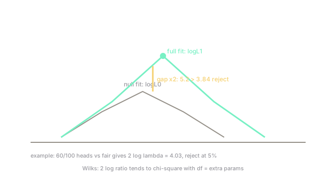
To compare two nested models, fit both and weigh the gap. Twice the log lift over the smaller model tells you whether the extra knobs earned it.

The constrained peak sits below the full peak, and twice the log gap at 5.2 clears the 3.84 chi-square cutoff to reject

Why Does This Exist?

"Does this feature help?" means comparing a small model against one with extra knobs. The big model always fits training data at least as well, so raw fit cannot decide. You need the price of flexibility.

The likelihood ratio $\\lambda = L(\\hat\\theta_0)/L(\\hat\\theta)$ pays exactly that price. Wilks says $2\\log\\lambda^{-1} = 2(\\ell_1 - \\ell_0)$ tends to $\\chi^2_d$ with $d$ extra parameters. It extends hypothesis testing with the workhorse behind ANOVA, deviance, and many A/B model checks, assuming the MLE machinery in maximum likelihood estimation.

The one idea you need first

Log-likelihood $\\ell(\\theta)$ scores parameters by fit; its max is the MLE. The gap $\\ell_1 - \\ell_0 \\geq 0$ measures what the extra knobs bought. Doubling turns the gap into chi-square units.

Think of It Like This

Two tailors, one surcharge

Two tailors fit you a suit. The standard tailor uses your size; the bespoke tailor adds shoulder, drape, and cuff knobs and fits slightly better. The question is whether the better fit beats the bespoke surcharge.

Twice the log gap is the fit improvement in standard currency; the $\\chi^2$ cutoff is the surcharge for $d$ knobs (3.84 for one at 5%). Where it stops: tailors can overfit fabric quirks, and so can models, which is why the cutoff grows with $d$ .

How It Actually Works

Fit full $\\hat\\theta$ and constrained $\\hat\\theta_0$ , compute $D = 2(\\ell(\\hat\\theta) - \\ell(\\hat\\theta_0))$ , reject $H_0$ when $D > \\chi^2_{d,1-\\alpha}$ . Needs nesting ( $H_0$ restricts $H_1$ ), interior optima, and enough data for $\\chi^2$ asymptotics. Siblings: Wald uses $\\hat\\theta$ distance over standard error; score uses slope at $H_0$ . All three agree asymptotically; LRT is the most invariant to parameterization.

Worked example

Hundred flips, 60 heads, test fair $p = 0.5$ . Full MLE $\\hat p = 0.6$ : $\\ell_1 = 60\\log 0.6 + 40\\log 0.4 \\approx -67.30$ . Null: $\\ell_0 = 100\\log 0.5 \\approx -69.31$ . Gap $2.01$ , doubled $D \\approx 4.03 > 3.84$ : reject fair at 5%. Wald check: $(0.6-0.5)/0.05 = 2.0$ , borderline the same verdict. One extra parameter, one 3.84 bar, cleared by 0.19.

Code

1import numpy as np2
3k, n = 60, 1004ell1 = k * np.log(k / n) + (n - k) * np.log(1 - k / n)5ell0 = n * np.log(0.5)6print(round(float(2 * (ell1 - ell0)), 2))  # -> 4.03

Doubled gap 4.03 clears 3.84. Same data, same verdict as the hand calculation.

Watch Out For

Testing non-nested models with Wilks

Comparing a Poisson against a negative binomial by $\\chi^2$ cutoff misfires when neither nests the other: the limit law is not $\\chi^2$ and the cutoff is fiction. Symptom: wildly significant verdicts that vanish under cross-validation.

Use Vuong, information criteria, or held-out likelihood for non-nested choices. Reserve Wilks for true nesting.

Testing on the boundary

Testing variance $= 0$ or mixture weight $= 0$ parks $H_0$ on the parameter edge, halving the limit law (e.g. $\\tfrac{1}{2}\\chi^2_0 + \\tfrac{1}{2}\\chi^2_1$ ). Naive $\\chi^2_d$ cutoffs run conservative and miss real effects.

Use boundary-corrected mixtures or bootstrap the null. If the null sits on an edge, distrust textbook cutoffs.

The Quick Version

LRT doubles the log-likelihood gap between nested fits and compares to $\\chi^2_d$ .
One extra parameter at 5% means clearing 3.84.
60 of 100 heads gives 4.03 and rejects fair, matching the Wald $z = 2.0$ .
Wald and score are asymptotic siblings; LRT respects reparameterization best.
Non-nested models need Vuong or held-out checks, not Wilks.
Boundary nulls halve the limit law; correct or bootstrap.