Math

Hypothesis Testing

A procedure for asking whether chance alone could plausibly have produced what you observed — and a p-value is the answer to that question, not to the one you probably wanted.

A p-value asks how often pure chance would produce a gap this large, and a two-point accuracy difference on a thousand examples falls comfortably inside what chance already does

Why Does This Exist?

Your new model scores two points higher. Is that a real improvement or a lucky test set?

You cannot answer by staring at the numbers, and the cost of getting it wrong runs both ways: ship a model that is no better and you have spent a deployment for nothing; discard one that genuinely is better and you have thrown away a real gain. Hypothesis testing is the formal procedure for making that call, and it is what sits underneath every A/B test and every "statistically significant" claim in a paper.

The reason it needs its own page rather than a formula is that the p-value answers a different question from the one most people think it answers. It is not the probability your result is a fluke, and it is not the probability the null hypothesis is true. Those misreadings drive real decisions, so the distinction is worth the page.

Think of It Like This

A coin you suspect is loaded

Someone hands you a coin and claims it is fair. You flip it ten times and get eight heads.

You do not start by asking "is the coin loaded?" — you cannot answer that directly. Instead you ask a question you can answer: if the coin really were fair, how often would ten flips give eight or more heads? That is a calculation, and the answer is about 5.5%.

Now you have a decision, not a proof. Eight heads is on the unusual side for a fair coin, but not extraordinary — it happens about one time in eighteen. So you either accept that fairness is still plausible, or you decide the evidence is strong enough to act on. Both are defensible, and neither is certainty.

Two features of this reasoning matter more than the arithmetic. You assumed fairness and asked whether the data embarrasses that assumption — you never computed the probability the coin is loaded. And "not embarrassing enough" is not the same as "the coin is fair"; ten flips simply cannot detect a mild bias.

How It Actually Works

The procedure has five steps and they run in this order for a reason.

State the null hypothesis $H_0$ — the boring explanation, usually "no difference". And the alternative $H_1$ .
Choose $\alpha$ , your tolerance for false alarms, before looking at the data. Conventionally 0.05.
Compute a test statistic — a single number measuring how far the data sits from what $H_0$ predicts.
Compute the p-value — the probability of a statistic at least this extreme if $H_0$ were true.
Decide. If $p < \alpha$ , reject $H_0$ . Otherwise fail to reject.

What a p-value is, precisely

p = P(\text{data at least this extreme} \mid H_0 \text{ true})

In plain words: assuming there is no real effect, how often would chance alone produce a result this striking?

Read the conditional carefully, because the direction is the whole thing. It is $P(\text{data} \mid H_0)$ , not $P(H_0 \mid \text{data})$ . Three specific things a p-value is therefore not:

Not the probability that $H_0$ is true. Getting that requires a prior and Bayes' theorem.
Not the probability your result is a fluke.
Not a measure of effect size. A microscopic, useless difference produces a tiny p-value given enough data.

Two ways to be wrong

Type I error — rejecting a true $H_0$ . A false positive. Its rate is $\alpha$ , which you chose.
Type II error — failing to reject a false $H_0$ . A false negative, rate $\beta$ . Power is $1 - \beta$ : the chance of detecting a real effect.

The trade is unavoidable. Lowering $\alpha$ to reduce false alarms raises $\beta$ and costs you power. The only way to improve both at once is more data.

This is why "not significant" must never be reported as "no difference". An underpowered test that returns nothing has measured nothing, and with the sample sizes typical of ML evaluation, underpowered is the normal state.

Failing to reject is not accepting

$H_0$ is never proven. You either have enough evidence against it or you do not, and "not enough" covers both "there is no effect" and "there is an effect and my test was too weak to see it". Distinguishing those requires a power calculation, or a confidence interval — which tells you what effect sizes remain plausible, and is strictly more informative than the p-value.

Which test, for ML work

Two proportions, independent samples — two-proportion z-test. Comparing accuracy across separate test sets.
Two proportions, same examples — McNemar's test. This is the right one for comparing two models on one test set, and it is much more powerful because it looks only at the examples where the models disagree, which is where the information about the difference lives.
Two means — the t-test, or Welch's variant when the variances differ. Welch is the safer default.
No distributional assumption — a permutation test. Shuffle the labels many times and see how often chance beats your observed gap. Assumption-free and always available.

Worked example

Model A gets 87% and model B gets 89%, each on 1,000 examples. $H_0$ is that their true accuracies are equal.

Pool the two under $H_0$ — if they are the same, the best estimate uses all the data:

\hat p = \frac{870 + 890}{2000} = 0.88

The standard error of the difference:

\text{SE} = \sqrt{\hat p(1-\hat p)\left(\tfrac{1}{n_A} + \tfrac{1}{n_B}\right)} = \sqrt{0.88 \times 0.12 \times 0.002} = \sqrt{0.00021} \approx 0.01453

The test statistic:

z = \frac{0.89 - 0.87}{0.01453} \approx 1.376

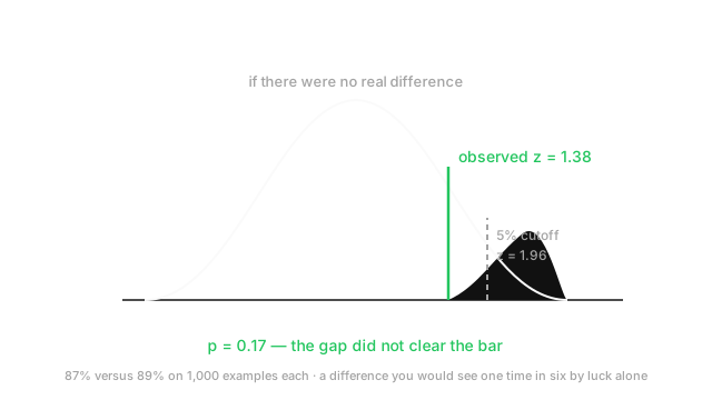
Since 1.376 is below the 1.96 cutoff, this does not reach significance. The two-sided p-value is $2 \times (1 - \Phi(1.376)) \approx 0.169$ .

In plain words: if the two models were genuinely equally good, you would see a gap this large about 17% of the time — roughly one experiment in six. That is far too common to treat as evidence.

Note how this agrees with the confidence-interval view: 87% ± 2.1 and 89% ± 2.1 overlap heavily, and the test confirms the same conclusion. They are one calculation.

What would settle it? Holding the 2-point gap fixed and solving for the $n$ that pushes $z$ past 1.96 gives roughly $n \approx 2000$ per model — so about double the data, and that is only to reach the threshold, not to have decent power.

Show Me the Code

1import numpy as np2from scipy import stats3
4
5def two_proportion_z(x1: int, n1: int, x2: int, n2: int) -> tuple[float, float]:6    p_pool = (x1 + x2) / (n1 + n2)                        # pooled under H07    se = np.sqrt(p_pool * (1 - p_pool) * (1 / n1 + 1 / n2))8    z = (x2 / n2 - x1 / n1) / se9    return float(z), float(2 * (1 - stats.norm.cdf(abs(z))))10
11
12z, p = two_proportion_z(870, 1000, 890, 1000)13print(round(z, 3), round(p, 3))            # -> 1.376 0.169  not significant14
15# Doubling the data on the same 2-point gap barely clears the bar.16print(np.round(two_proportion_z(1740, 2000, 1780, 2000), 4))   # -> [1.946 0.0517]17
18# Paired case: same test set, so use McNemar on the DISAGREEMENTS only.19# 40 examples B got right and A wrong; 20 the other way.20print(round(float(stats.binomtest(40, 60, 0.5).pvalue), 4))     # -> 0.0154  significant

The z of 1.376 and p of 0.169 match the hand calculation. The last line is the important one: the same 2-point gap, analysed as paired data, reaches significance — because pairing removes the variance the models share.

Watch Out For

Reading a p-value as the probability you are wrong

"p = 0.03, so there is a 3% chance this is a fluke" is the single most common statistical error in technical writing, and it inverts the conditional.

$P(\text{data} \mid H_0)$ is not $P(H_0 \mid \text{data})$ . Converting between them requires a prior on how likely the effect was to begin with, and when that prior is low the difference is enormous. If only 10% of your candidate improvements are genuinely real — a realistic rate for hyperparameter tweaks — then among results significant at $p = 0.05$ with 80% power, roughly a third are false positives. Not 5%.

That is the same base-rate arithmetic as a rare-disease test, and it explains why "significant" findings so often fail to replicate.

Two practical habits. Report the effect size and its confidence interval, not just the p-value: "recall improved 1.5 points, 95% CI [0.2, 2.8]" is a statement a reader can act on, and it also makes clear when a significant result is too small to matter. And treat significance as a filter, not a conclusion — the question after "is it real" is always "is it big enough to be worth the deployment".

Testing repeatedly and stopping when it turns significant

Peeking at results as data accumulates and stopping the moment $p < 0.05$ guarantees a false positive eventually, even with no real effect at all.

The reason is that the p-value fluctuates as data arrives. Check it once and your false-positive rate is the 5% you chose. Check it after every hundred observations and you are running many correlated tests, and the chance of crossing the threshold at some point approaches 1. Continuous monitoring of a fixed-sample test can push the effective false-positive rate above 20%.

This is the most common failure in ML A/B testing, and it does not feel like cheating — it feels like being attentive. The dashboard updates, someone notices the line has crossed, and the experiment is called.

Three correct approaches. Fix the sample size in advance from a power calculation, and do not look until you reach it. Use a sequential test designed for continuous monitoring — group sequential methods with alpha spending, or a Bayesian approach where updating as data arrives is legitimate by construction. Or use always-valid confidence sequences, which several experimentation platforms now implement for exactly this reason.

The related trap is the garden of forking paths: trying several metrics, segments, or windows and reporting the one that reached significance. That is multiple comparisons whether or not anyone counted the tests.

The Quick Version

State $H_0$ and $\alpha$ before looking at the data. Then compute a statistic, a p-value, and decide.
$p = P(\text{data this extreme} \mid H_0)$ . Not $P(H_0 \mid \text{data})$ , not the chance of a fluke, not an effect size.
Type I is a false positive at rate $\alpha$ ; Type II is a false negative at rate $\beta$ . Power is $1 - \beta$ .
Lowering $\alpha$ costs power. Only more data improves both.
"Not significant" is not "no difference." An underpowered test has measured nothing.
$H_0$ is never accepted, only not rejected.
A confidence interval is strictly more informative: it shows both significance and effect size.
Same test set → McNemar's test, which is far more powerful than treating the samples as independent.
Permutation tests need no distributional assumption and are always available.
87% vs 89% on 1,000 examples gives $z = 1.38$ , $p = 0.17$ — one experiment in six by chance.
Never peek and stop at significance. Fix $n$ in advance, or use a sequential method built for it.