Loss Landscape Geometry

The loss surface of a big network is full of saddles but short on bad valleys, which is why plain gradient steps keep reaching good solutions.

The loss surface holds a sharp narrow valley beside a wide flat basin, and a low-loss path connects two good solutions around the high barrier

Why Does This Exist?

Training a network means walking downhill on a surface with millions of dimensions, which sounds hopeless. Early intuition said the walk would get trapped in poor local valleys. Practice said otherwise: plain gradient methods routinely land somewhere good. Loss landscape geometry resolves the tension by describing what the surface actually contains.

Three findings carry most of the weight. High-dimensional surfaces are dominated by saddles (down in some directions, up in others) rather than true traps. The minima that remain divide into sharp ones that generalize poorly and flat ones that transfer better. And good solutions connect through low-loss paths, so the basin is more like a winding valley system than isolated pits. This page covers the surface; convexity covers the one-bottom case, and over-parameterized generalization covers why flatness transfers.

The one idea you need first

At any point, the gradient gives the downhill direction and the Hessian (matrix of second derivatives) describes curvature per direction. Positive curvature all around means a valley; mixed signs mean a saddle; near-zero curvature in many directions means a flat plain.

Think of It Like This

A mountain range crossed by high passes

Picture a vast range with almost no boxed-in crater lakes but countless high passes. A ball rolled downhill rarely gets stuck, because at each pass at least one direction still descends. It keeps crossing passes until it reaches a broad high valley with many campsites.

Some campsites sit on knife ridges: one step sideways and you fall off (sharp minima, poor transfer). Others sit on wide meadows: you can wander without climbing (flat minima, sturdy predictions). And the meadows connect: you can walk from one good camp to another without crossing a peak, staying low the whole way. The range looks threatening from afar and walks easily once you stop fearing craters that are not there.

How It Actually Works

Saddles dominate. In $n$ dimensions with random curvatures, the chance all $n$ directions curve upward is $2^{-n}$ : astronomically small for $n$ in the millions. So critical points where the gradient vanishes are overwhelmingly saddles with at least one escape direction. Gradient descent with a little noise slides off them, which is why high dimension helps rather than hurts.

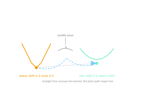
Flat versus sharp. Near a minimum $w^*$ , the loss grows like $\frac{1}{2}(w - w^*)^T H (w - w^*)$ with Hessian $H$ . Large eigenvalues mean steep walls: a small shift (like the train-to-test shift) raises the loss a lot. Small eigenvalues mean a wide basin where shifts cost little. Empirically, solutions found with small batches and moderate learning rates land flatter and test better than the sharp minima large batches prefer.

Mode connectivity. Take two independently trained solutions $w_1, w_2$ with low loss. The straight line between them usually crosses a high barrier, but a bent path (a polygonal chain with one kink) stays at low loss throughout. Good solutions form a connected low-loss manifold, not isolated pits.

Worked example

A two-dimensional toy with a saddle at the origin and a flat and a sharp minimum:

L(x, y) = x^2 - y^2 + 0.1x^4 + 5(y - 2)^2 x^2

At $(0,0)$ : Hessian $\text{diag}(2, -2)$ , mixed signs, a saddle. Gradient descent from $(0.1, 0.1)$ with step $0.1$ moves $y$ away from zero within about $20$ steps (the $-2$ curvature pushes outward) while $x$ shrinks. Contrast two minima of $L_1(w) = 50w^2$ (sharp, curvature $100$ ) and $L_2(w) = 0.5w^2$ (flat, curvature $1$ ): a shift of $0.3$ raises the sharp loss by $50 \times 0.09 = 4.5$ but the flat one by only $0.5 \times 0.09 = 0.045$ , a hundredfold difference in sensitivity.

Code

1def sharp_loss(w: float) -> float:2    return 50.0 * w * w  # curvature 1003
4
5def flat_loss(w: float) -> float:6    return 0.5 * w * w  # curvature 17
8
9for shift in (0.1, 0.3, 0.5):10    print(shift, round(sharp_loss(shift), 3), round(flat_loss(shift), 4))11# -> 0.1 0.5 0.00512# -> 0.3 4.5 0.04513# -> 0.5 12.5 0.125

The sharp basin penalizes the same shift a hundred times harder, which is the flat-minima argument in one table.

Watch Out For

Treating every stationary point as a trap

Visualizing a one-dimensional slice through the surface shows valleys everywhere, and each looks like a trap. But a point that is a minimum along your slice is usually a saddle in full space, with escape directions your slice missed. Never diagnose trapping from a 1-D or 2-D plot alone.

Chasing flatness past the point of returns

Very flat regions can be flat because the model stopped using capacity (dead units, saturated blocks), not because it found a sturdy solution. If sharpness tools report near-zero curvature everywhere including on training data the model fits poorly, suspect underuse before celebrating generalization.

The Quick Version

Big-network surfaces are rich in saddles and poor in bad valleys, since all-up curvature has chance $2^{-n}$ .
Noise plus gradient steps escape saddles through their downhill directions.
Flat minima tolerate train-test shifts; sharp ones amplify them a hundredfold in the worked example.
Good solutions connect via bent low-loss paths even when the straight line crosses a barrier.
Small batches and moderate steps bias toward flatter, better-transferring solutions.
One-dimensional slices mislead: minima on the slice are usually saddles in full space.