Math

Kullback–Leibler Divergence

How many extra bits you pay for encoding reality with the wrong model — and because the penalty is charged against reality's probabilities, not the model's, swapping the two gives a different number.

KL divergence measures the cost of using one distribution in place of another, and because the cost is weighted by the first distribution's probabilities, swapping the arguments changes the answer

Why Does This Exist?

You need a number that says how wrong a distribution is, and the obvious candidates do not work.

Subtracting probabilities elementwise gives you a vector, not a score. Taking a Euclidean distance between probability vectors treats a 0.5 → 0.4 change the same as a 0.1 → 0.0 change, when the second one is catastrophic and the first is a rounding error — a model that assigns zero probability to something that happens is infinitely wrong, and no distance built from subtraction can express that.

KL divergence is the measure that gets this right, and three things in modern ML are literally it:

The KL term in a VAE loss pulls the encoder's output distribution toward the prior. It is the second half of the ELBO, and the entire reason a VAE's latent space is usable for sampling rather than being a scattered lookup table.
DPO and RLHF regularisation keep a fine-tuned policy from drifting too far from the reference model. The penalty is a KL divergence, and the coefficient on it, usually written $\beta$ , is the single most consequential hyperparameter in preference tuning.
Knowledge distillation trains a small model to match a large one's full output distribution rather than its top answer. The loss is a KL divergence, and matching the distribution is why distillation transfers more than relabelling would.

There is also a fact that reframes classification: minimising cross-entropy is minimising a KL divergence. The gap between them is the data's own entropy, which no model can change. Every classifier you have trained was doing this page's arithmetic.

Think of It Like This

Paying for a phrasebook printed for the wrong city

You are compressing messages. You have a codebook that assigns short codes to things it expects often and long codes to things it expects rarely — the standard trick, and the optimal codebook for a given set of frequencies is exactly what entropy measures.

Now the codebook was built for the wrong place. It was printed for a city where 90% of messages are "fine, thanks", so that phrase gets a one-syllable code and everything else gets a long one. You take it somewhere that says "fine, thanks" only half the time.

Every message still transmits. Nothing breaks. But you are now spending long codes on things that happen constantly, and the average message costs more than it had to. KL divergence is exactly that excess, measured in bits per message.

Two features of the analogy carry over precisely, and they are the two things people get wrong:

It is never negative. The wrong codebook can tie the right one — if it happens to have the same frequencies — but it can never beat it. Zero means identical, and nothing is below zero.

It is not symmetric, and the asymmetry has a direction with meaning. The cost is averaged over the messages you actually send, not the ones the codebook expected. A codebook that is wrong about something you never say costs you nothing. A codebook that assigns a long code to your most common phrase costs you constantly. Swap which place is real and which is the codebook, and the bill changes.

The hard case makes it stark: if the codebook has no code at all for something you say, the message cannot be sent. That is the infinite case, and it is not a mathematical curiosity — it is the most common way this quantity blows up in code.

How It Actually Works

Write $P$ for the distribution that is real — the data, the true labels, the target — and $Q$ for the one standing in for it, usually your model. Over a discrete set of outcomes:

D_{\mathrm{KL}}(P \parallel Q) = \sum_x P(x) \log \frac{P(x)}{Q(x)}

In plain words: for each outcome, take the log of how much the two distributions disagree about it, then average those disagreements weighted by how often that outcome actually happens. That weighting is where all the asymmetry comes from.

For continuous variables the sum becomes an integral, exactly as in integrals in probability:

D_{\mathrm{KL}}(P \parallel Q) = \int p(x) \log \frac{p(x)}{q(x)}\, dx

Read $\parallel$ as "relative to". The left argument is reality; the right is the stand-in.

Its relationship to cross-entropy

Split the log and the identity falls out:

D_{\mathrm{KL}}(P \parallel Q) = \underbrace{-\sum_x P(x) \log Q(x)}_{H(P, Q)} - \underbrace{\left(-\sum_x P(x) \log P(x)\right)}_{H(P)}

In plain words: divergence equals cross-entropy minus entropy. Cross-entropy is the total bill; entropy is the part that was unavoidable; KL is the avoidable excess.

This is why classification training does not need a KL term. Your targets $P$ are fixed, so $H(P)$ is a constant, so minimising cross-entropy and minimising KL differ by a number that has no gradient. Cross-entropy is used because it is the cheaper of two identical objectives.

It also explains the floor. Cross-entropy loss does not go to zero on real data — it goes to $H(P)$ . A validation loss that stalls at 0.3 on a genuinely ambiguous labelling task has not stalled; it has arrived.

Three properties that matter, and one that is missing

Non-negativity. $D_{\mathrm{KL}}(P \parallel Q) \ge 0$ , with equality only when the distributions match everywhere. This follows from Jensen's inequality — for the concave $\log$ , the average of the logs is at most the log of the average — and it is the same inequality that makes the ELBO a lower bound. If you have wondered why the ELBO is called a bound and what guarantees the direction, this is the guarantee.

Asymmetry. $D_{\mathrm{KL}}(P \parallel Q) \ne D_{\mathrm{KL}}(Q \parallel P)$ in general. It is a divergence, not a distance.

No triangle inequality. You cannot chain it. " $Q$ is close to $P$ and $R$ is close to $Q$ " implies nothing reliable about $R$ and $P$ .

The missing property is symmetry, and when you genuinely need a symmetric measure the standard answer is Jensen–Shannon divergence: average both directions against the mixture $M = \tfrac{1}{2}(P + Q)$ . It is symmetric, always finite, and its square root is a true metric. Reach for it when you are reporting a distance between distributions rather than optimising one.

The asymmetry is a modelling choice

Which direction you minimise changes what your model does, and this is not subtle.

Forward KL, $D_{\mathrm{KL}}(P \parallel Q)$ — mass covering. The weights are $P(x)$ , so the penalty is large wherever the data has mass and the model does not. A model minimising this cannot afford to ignore any real region, so it spreads out to cover everything, including the gaps between modes. Maximum likelihood is this direction, which is why an over-simple density model trained by MLE produces blurry averages: it is covering two modes by putting mass between them.

Reverse KL, $D_{\mathrm{KL}}(Q \parallel P)$ — mode seeking. The weights are $Q(x)$ , so regions where the model puts no mass are free, however real they are. A model minimising this picks one mode and commits. Variational inference minimises this direction, which is why a variational posterior is characteristically too confident: it found one mode and reported its width, not the full posterior's.

Neither is correct in general. Choose deliberately: forward KL to avoid missing anything, reverse KL to get a sharp answer you can sample from.

Worked example

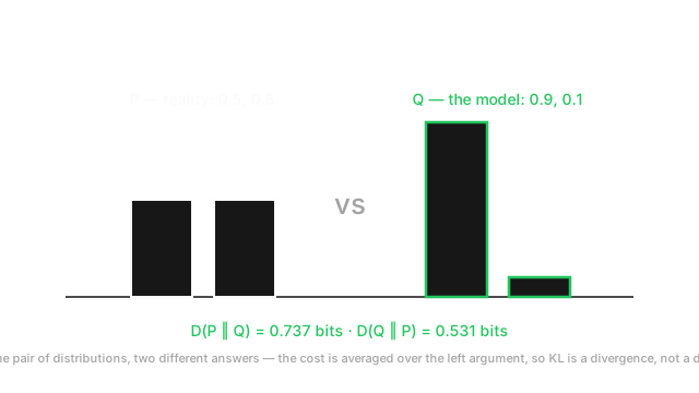
Two distributions over two outcomes. $P = (0.5,\ 0.5)$ — genuinely uncertain. $Q = (0.9,\ 0.1)$ — confidently wrong. All logs base 2, so the answers are in bits.

Forward direction, weighting by $P$ :

D_{\mathrm{KL}}(P \parallel Q) = 0.5 \log_2 \frac{0.5}{0.9} + 0.5 \log_2 \frac{0.5}{0.1}

The two terms are $0.5 \times (-0.8480) = -0.4240$ and $0.5 \times 2.3219 = 1.1610$ , giving

D_{\mathrm{KL}}(P \parallel Q) = 0.7370 \text{ bits}

Note that the first term is negative. Individual terms can be negative — $Q$ is closer to right than $P$ on that outcome — while the total cannot.

Now swap:

D_{\mathrm{KL}}(Q \parallel P) = 0.9 \log_2 \frac{0.9}{0.5} + 0.1 \log_2 \frac{0.1}{0.5} = 0.7632 - 0.2322 = 0.5310 \text{ bits}

0.7370 against 0.5310. Same pair of distributions, two different answers, differing by 39%. Anyone treating this as a distance has already made an error.

Check it against the cross-entropy identity. $H(P) = 1$ bit exactly, since $P$ is uniform over two outcomes. Cross-entropy:

H(P, Q) = -\left(0.5 \log_2 0.9 + 0.5 \log_2 0.1\right) = 0.0760 + 1.6610 = 1.7370 \text{ bits}

And $1.7370 - 1 = 0.7370$ , matching the forward divergence exactly. The identity is not an approximation.

One more case, because it is the one that breaks code. Let $Q = (1.0,\ 0.0)$ . The second term of the forward divergence is $0.5 \log_2 (0.5 / 0)$ , which is infinite. A model that rules out something that happens half the time is infinitely wrong, and the arithmetic says so. Meanwhile $D_{\mathrm{KL}}(Q \parallel P)$ is a finite $1$ bit, because the direction weighted by $Q$ never visits the outcome $Q$ assigned zero to.

Show Me the Code

1import numpy as np2
3EPS = 1e-12  # guards log(0); see the pitfall below for why this is not enough4
5
6def kl_bits(p: np.ndarray, q: np.ndarray) -> float:7    """KL(p || q) in bits. Both args shape (k,), each summing to 1."""8    p, q = np.asarray(p, dtype=np.float64), np.asarray(q, dtype=np.float64)9    mask = p > 0                                   # 0 * log 0 contributes 0, not nan10    return float(np.sum(p[mask] * np.log2(p[mask] / (q[mask] + EPS))))11
12
13P, Q = np.array([0.5, 0.5]), np.array([0.9, 0.1])14print(round(kl_bits(P, Q), 4))                     # -> 0.73715print(round(kl_bits(Q, P), 4))                     # -> 0.531   not the same number16
17cross_entropy = -float(np.sum(P * np.log2(Q)))     # 1.73718entropy = -float(np.sum(P * np.log2(P)))           # 1.019print(round(cross_entropy - entropy, 4))           # -> 0.737   identity confirmed20
21print(round(kl_bits(P, np.array([1.0, 0.0])), 1))  # -> 18.9   epsilon, not infinity

The last line is the important one. The true answer is infinite; the epsilon turns it into 18.9 bits, and 18.9 is a finite number that an optimiser will happily try to reduce. The guard did not fix the problem, it hid it.

Watch Out For

Adding epsilon inside the log and calling the zero problem solved

log(q + 1e-12) stops the nan, and that is the entire extent of what it does.

You have replaced an infinity with about 19 bits, and 19 bits is a live gradient. One outcome that your model assigned near-zero probability to now dominates the loss and the update, and training either destabilises or spends its capacity on that single point. The symptom is a loss that spikes on particular batches and a model that never converges cleanly, with no nan to point at.

Worse, the value depends on the epsilon rather than on the data. Change 1e-12 to 1e-8 and your reported divergence changes by a third, on identical inputs. Any number you publish is partly a function of a constant you picked arbitrarily.

What to do instead, in order of preference:

Work in log space end to end. Take log-probabilities as input and use torch.nn.functional.kl_div with log_target=True, or scipy.special.rel_entr on the probabilities. These are built to keep the subtraction stable rather than patching the input.
Make zeros impossible at the source. A softmax output is never exactly zero in principle; if yours is, it underflowed, and the fix is numerical stability in the softmax, not an epsilon downstream.
Smooth the target deliberately. Label smoothing at $\varepsilon = 0.1$ is a documented modelling decision with a known effect on calibration. An epsilon buried in a utility function is neither.
Switch measures if zeros are genuine. If your distributions really do have disjoint support — comparing empirical histograms, say — KL is the wrong tool. Jensen–Shannon divergence stays finite by construction.

Add the epsilon outside the log where it belongs, or add it nowhere. And keep the p > 0 mask: where $P(x) = 0$ the term is genuinely zero, because $\lim_{p \to 0} p \log p = 0$ , and masking is exact rather than approximate.

Reading a KL number without saying which direction it was, or what the base is

Two ambiguities in one quantity, and both produce numbers that are not comparable to anything.

Direction. Library signatures disagree. scipy.stats.entropy(pk, qk) computes $D_{\mathrm{KL}}(pk \parallel qk)$ , first argument as reality. PyTorch's kl_div(input, target) computes $D_{\mathrm{KL}}(\text{target} \parallel \text{input})$ — the second argument is reality, and input is expected to already be log-probabilities. The two conventions are reversed, and swapping them silently trains a mode-seeking objective when you specified a mass-covering one. The result is not an error; it is a model that quietly collapses to one mode. Verify the direction with an asymmetric pair like the worked example above the first time you use any KL function, in any library.

Base. Base 2 gives bits, base $e$ gives nats, and the ratio is $\ln 2 \approx 0.693$ . Every deep learning library uses nats. A KL value of 0.5 means something different in each convention, and a $\beta$ coefficient tuned under one is mis-scaled by 44% under the other. When a paper's regularisation coefficient does not reproduce, this is one of the first things to check.

The reporting habit that avoids both: write the direction explicitly and name the unit. " $D_{\mathrm{KL}}(\text{posterior} \parallel \text{prior}) = 0.42$ nats", not "KL = 0.42".

The Quick Version

KL divergence measures the excess cost of using $Q$ where $P$ is real, in bits or nats per observation.
$D_{\mathrm{KL}}(P \parallel Q) = \sum_x P(x) \log \frac{P(x)}{Q(x)}$ . The weights are $P$ 's probabilities, and that is the source of every property below.
It equals cross-entropy minus entropy, so minimising cross-entropy is minimising KL. The unavoidable $H(P)$ is why validation loss has a non-zero floor.
Always non-negative, zero only for identical distributions. Non-negativity comes from Jensen's inequality, the same one that makes the ELBO a lower bound.
Not symmetric and no triangle inequality. It is not a distance. Use Jensen–Shannon divergence when you need one.
Forward KL is mass-covering and produces blurry averages; reverse KL is mode-seeking and produces overconfident posteriors. MLE is forward, variational inference is reverse.
It is infinite when $Q$ assigns zero probability to something $P$ does not. Epsilon-guarding hides this rather than solving it.
Library argument orders and log bases disagree. State the direction and the unit whenever you report a value.