Math

Norms

A single number for how big a vector is — and there is more than one reasonable way to measure that, which is why the choice changes what your model learns.

Each norm draws a different shape through the vectors it calls length one: L2 a circle, L-infinity a square, and L1 a diamond whose corners sit on the axes, which is why L1 pushes coordinates to exactly zero

Why Does This Exist?

"The gradient exploded" is a statement about a norm. So is "clip at 1.0", "weight decay of 0.01", and "these two embeddings are close". Each one reduces a vector of thousands of numbers to a single measure of size, and every time, a specific norm was chosen — usually silently, usually L2.

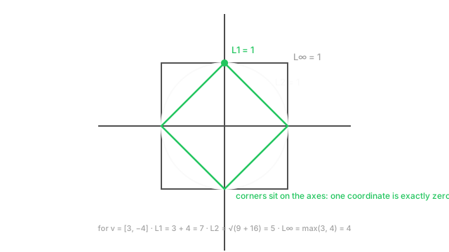
That choice is not cosmetic. Swap L2 for L1 in a regularisation penalty and you do not get a slightly different model; you get a model with exactly zero in most of its coefficients instead of small nonzero values everywhere. Same intent, different geometry, qualitatively different outcome. Understanding why is the point of this page, and the diagram above is most of the answer.

There is also a concrete numerical trap here that costs people real debugging time: the obvious way to compute an L2 norm overflows on inputs whose true norm is perfectly representable. It is worth knowing before you write the one-liner.

Think of It Like This

Three honest answers to how far away it is

You are at one corner of a city grid and your destination is three blocks east and four blocks north. How far is it?

A pigeon says five blocks. It flies straight over the buildings, and by Pythagoras that diagonal is exactly 5. That is the L2 norm.

A taxi says seven blocks. It cannot drive through buildings, so it goes three east and four north, and seven is the real distance travelled. That is the L1 norm.

A project manager says four blocks. They only care about the longest leg, because that is the part that dominates the schedule. That is the L-infinity norm.

Nobody is wrong. They are answering under different constraints, and the shape of the constraint decides the answer. When you choose a norm in a loss function, you are choosing which of these three the optimiser is allowed to be.

How It Actually Works

A norm takes a vector and returns a single non-negative number. Any function calling itself a norm has to satisfy three properties, and they are worth knowing because they are what makes a norm usable as a penalty: it is zero only for the zero vector, scaling the vector scales the norm by the same factor, and the triangle inequality holds.

The family used almost everywhere is the p-norm:

\lVert v \rVert_p = \left( \sum_{i} |v_i|^p \right)^{1/p}

In plain words: raise the size of every component to the power $p$ , add them up, then take the $p$ -th root. Three values of $p$ cover nearly all practical use:

$p = 1$ , the L1 norm — just add the absolute values. Also called Manhattan or taxicab distance.
$p = 2$ , the L2 norm — the square root of the sum of squares. Ordinary straight-line length, and the default meaning of $\lVert v \rVert$ when no subscript is written.
$p \to \infty$ , the L-infinity norm — the largest absolute component. The sum gets dominated by its biggest term as $p$ grows, so only the maximum survives.

L2 is the default for a reason worth naming: it is the only p-norm that comes from a dot product, since $\lVert v \rVert_2 = \sqrt{v \cdot v}$ . That connection is what gives L2 angles, projections, and a smooth derivative everywhere except the origin. L1 and L-infinity have none of it.

Why the shapes matter more than the formulas

The diagram above draws the unit ball of each norm: the set of all vectors that norm calls length 1. L2 gives a circle, L-infinity a square, L1 a diamond.

Now the payoff. When you add a norm penalty to a loss, the optimiser is pushed toward small values of that norm — pressed inward against one of those shapes. And where a shape touches an axis decides what happens:

The L2 circle is smooth everywhere. It has no special points, so the solution it favours has all coordinates small and none of them exactly zero. This is shrinkage.
The L1 diamond has corners, and the corners sit precisely on the axes. A corner is where one coordinate is exactly zero. Because a corner is a much better place for a constrained optimum to land than a flat face, L1 solutions collapse coordinates to true zeros. This is sparsity, and it is a consequence of geometry, not of the formula looking different.

That is the whole L1-versus-L2 story. L1 gives you feature selection for free because its unit ball has spikes pointing along the axes. L2 gives you smooth, well-behaved shrinkage because its unit ball has no spikes at all.

The trade-off: L1's corners are exactly the points where the derivative does not exist, so L1 penalties need optimisers that tolerate a subgradient, and they are less smooth to train.

What gradient clipping actually clips

Clipping is the most common place a practitioner meets a norm directly. The rule is: compute the L2 norm of the gradient, and if it exceeds a threshold $c$ , rescale the whole gradient down so its norm is exactly $c$ .

g \leftarrow g \cdot \min\left(1, \frac{c}{\lVert g \rVert_2}\right)

In plain words: if the gradient is longer than allowed, shrink it to the allowed length; otherwise leave it alone. The crucial detail is that the direction is preserved — every component is scaled by the same factor. That is what separates norm clipping from value clipping, which caps each component independently and therefore changes which way the gradient points.

Worked example

Take $v = [3, -4]$ .

\lVert v \rVert_1 = |3| + |{-4}| = 7, \qquad \lVert v \rVert_2 = \sqrt{3^2 + 4^2} = 5, \qquad \lVert v \rVert_\infty = \max(3, 4) = 4

In plain words: the taxi drives 7, the pigeon flies 5, the longest single leg is 4. Three different numbers for the same vector, and notice they are ordered — L-infinity is never larger than L2, which is never larger than L1. That ordering holds in general and is a fast sanity check on any implementation.

To turn $v$ into a unit vector, divide by its L2 norm: $v / 5 = [0.6, -0.8]$ . Check: $0.36 + 0.64 = 1$ .

If you were clipping at $c = 2$ , the scale factor would be $2/5 = 0.4$ , giving $[1.2, -1.6]$ — same direction, length now exactly 2.

Show Me the Code

1import numpy as np2
3
4def clip_by_norm(g: np.ndarray, c: float) -> np.ndarray:5    # Scale every component by ONE factor, so the direction is untouched.6    return g * min(1.0, c / float(np.linalg.norm(g)))7
8
9v = np.array([3.0, -4.0])   # shape (2,)10print(np.linalg.norm(v, 1), np.linalg.norm(v), np.linalg.norm(v, np.inf))  # -> 7.0 5.0 4.011print(v / np.linalg.norm(v))          # -> [ 0.6 -0.8]   unit vector12print(clip_by_norm(v, 2.0))           # -> [ 1.2 -1.6]   length exactly 213
14# The naive formula overflows where linalg.norm does not.15big = np.array([1e200, 1e200], dtype=np.float64)16print(np.sqrt(np.sum(big**2)))        # -> inf   squaring overflowed first17print(np.linalg.norm(big))            # -> 1.414...e+200   correct

Seven, five and four, matching the hand calculation. The last two lines are the trap the next section is about.

Watch Out For

Writing the L2 norm as sqrt(sum(x**2))

The textbook formula translated directly into code is numerically fragile, and it fails in both directions.

float64 tops out around $1.8 \times 10^{308}$ . Square a component of $10^{200}$ and you get $10^{400}$ , which overflows to inf before the square root ever runs — so the norm returns inf even though the true answer, about $1.4 \times 10^{200}$ , is comfortably representable. In float32 the ceiling is only about $3.4 \times 10^{38}$ , so anything past roughly $2 \times 10^{19}$ overflows, and in float16 it happens at around 256.

The mirror image is just as real: components around $10^{-200}$ square to $10^{-400}$ , which underflows to exactly zero, and the norm reports 0 for a vector that is not zero. Then you divide by it.

np.linalg.norm and every BLAS implementation avoid this by factoring out the largest absolute component first, squaring only ratios that are all at most 1, and multiplying the scale back afterwards. Use the library function. The hand-rolled version is fine right up until real data reaches it, which is the worst possible time to find out.

Clipping over the wrong scope

Gradient clipping needs a scope, and the answer changes completely depending on what you pick. Clipping the global norm across all parameters at once treats the model as one long vector and preserves the relative scale between layers. Clipping per parameter tensor rescales each layer independently, which changes the balance between them.

Neither is wrong, but they are different algorithms, and papers frequently do not say which they used. Reproducing a result with the other one gives noticeably different training dynamics and a tuned threshold that no longer transfers — the global norm over a large model is much larger than any individual tensor's norm, so a threshold of 1.0 means something very different in each case.

There is a subtler version inside a single tensor. Computing a norm over a batch of gradients without specifying axis collapses the whole batch to one number; passing axis=1 gives one norm per example. If you meant per-example clipping — as differentially private training requires — the missing axis silently gives you batch-level clipping instead, and the privacy guarantee you were relying on does not hold.

The Quick Version

A norm reduces a vector to one non-negative number describing its size.
L1 sums absolute values, L2 is the square root of the sum of squares, L-infinity takes the largest component.
$\lVert v \rVert_\infty \le \lVert v \rVert_2 \le \lVert v \rVert_1$ always. Useful as a sanity check.
L2 is the default because it comes from a dot product, which is what gives it angles, projections, and smooth derivatives.
Unit balls explain the behaviour: L1's diamond has corners on the axes, so L1 drives coordinates to exactly zero. L2's circle is smooth, so it only shrinks them.
Gradient clipping rescales by the L2 norm and preserves direction. Value clipping does not.
Never compute an L2 norm as sqrt(sum(x**2)) — it overflows and underflows. Use the library function.
Clipping scope matters: global versus per-tensor versus per-example are three different algorithms.