Numerical Integration
Estimating integrals without antiderivatives: weighted sums of function values that converge to the area. Most ML integrals end here, not in closed form.
Why Does This Exist?
Most integrals in ML have no closed form: Bayesian posteriors, expected losses over continuous noise, partition functions. Analytic integration, taught in integration and area, handles the textbook cases; everything else needs numerical integration (quadrature): approximate by a weighted sum of function values at chosen points.
The design space is one trade: where to put the points and how to weight them. Trapezoids join values with straight lines (cheap, robust). Simpson fits parabolas (exact for cubics and below). Gaussian quadrature optimises both points and weights (maximum exactness per evaluation). Monte Carlo scatters points randomly (dimension-proof, slow convergence). Expectations over distributions connect in Monte Carlo methods.
The one idea you need first
A Riemann sum slices into panels and totals rectangle areas: the integral is its limit as panels thin. Quadrature rules are smarter panels: trapezoid averages the two endpoint heights per panel, Simpson weights endpoint-midpoint-endpoint as -- per double panel. Same limit, far fewer panels.
Think of It Like This
Surveying a curved field with straight fences
A field's boundary curves, but your measuring tape runs straight between posts. Plant posts at intervals and join them with straight fence runs (trapezoid): each run cuts or overshoots the true boundary, and the errors shrink as posts multiply.
Simpson upgrades the fence to flexible rails bent through three posts at a time, hugging the curve. Gaussian quadrature hires the surveyor to choose post positions optimally for the terrain instead of spacing them evenly. Monte Carlo throws darts and counts landings: crude per dart, unbeatable when the field has a hundred dimensions and fences stop working.
How It Actually Works
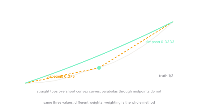
On with and two panels (, points ):
- Trapezoid: . Error : overshoots because straight tops sit above the convex curve.
- Simpson: . Exact: parabolas reproduce quadratics, so the only error is rounding.
Same three function values, 0.375 versus 0.3333 against truth . The weights did all the work. Gaussian quadrature with points integrates degree- polynomials exactly; Monte Carlo's rate ignores dimension, which is why hundred-dimensional expectations sample rather than grid.
Worked example
Integrate on (truth ). The trapezoid computation above gives , off by . Halve to (points ): . Error falls , a factor of 4 for halved : the rate made visible. Simpson needed no refinement at all.
Code
The point is the check: implement both rules and confirm the error ratio on refinement.
def trapezoid(f: list[float], h: float) -> float: return h * (f[0] / 2 + sum(f[1:-1]) + f[-1] / 2)
def simpson(f0: float, f1: float, f2: float, h: float) -> float: return h / 3 * (f0 + 4 * f1 + f2) # one double panel
vals = [0.0, 0.25, 1.0] # x squared at 0, 0.5, 1print(trapezoid(vals, 0.5)) # -> 0.375print(round(simpson(0.0, 0.25, 1.0, 0.5), 4)) # -> 0.3333Watch Out For
Pushing Newton-Cotes to high order
Simpson (order 2) behaves; order-8 Newton-Cotes on evenly spaced points oscillates wildly between nodes (Runge's phenomenon) with exploding weights that amplify function noise. High accuracy comes from composite low-order rules on more panels, or Gaussian points, never from cranking one panel's degree.
Gridding a high-dimensional integral
A 10-point grid in 20 dimensions needs evaluations: the curse in its purest form. Quadrature grids die past 4 or 5 dimensions. Switch to Monte Carlo (or quasi-Monte Carlo, or variational bounds) when dimensions pile up, and distrust any grid-based estimate that "worked in 2D".
The Quick Version
- Quadrature replaces integrals with weighted sums of function values at chosen points.
- Trapezoid on gives 0.375; Simpson gives exactly from the same three values.
- Halving trapezoid panels quarters the error: the rate in action.
- Gaussian quadrature maximises exactness per evaluation; Monte Carlo ignores dimension at .
- Composite low-order rules beat single high-order ones; grids die in high dimensions.