Math

Expectation, Variance and Covariance

Three summary numbers: where the values centre, how far they scatter from that centre, and whether two of them scatter together.

$Two datasets can share an identical average and still be nothing alike: the mean says where the centre is and the variance says how far from it the values actually fall$

Two datasets can share an identical average and still be nothing alike: the mean says where the centre is and the variance says how far from it the values actually fall

Why Does This Exist?

A mean on its own is close to useless, and machine learning is full of places where relying on one costs you.

Two models both average 91% accuracy across five folds. One scored 90, 91, 91, 91, 92; the other scored 78, 85, 95, 98, 99. Identical means, and only one of them is something you would deploy. The second is telling you it depends heavily on which data it sees, and no amount of staring at the average will reveal that.

Variance is the number that separates them, and it runs through the field: the bias-variance trade-off, batch normalisation, weight initialisation schemes, Adam's second-moment estimate, error bars on any benchmark you should believe. Covariance extends it to pairs and is what feature correlation, multicollinearity, and PCA are all built on.

There is also a specific numerical trap here that is genuinely famous. The algebraically tidy one-pass formula for variance is unusable on real data with large means, and it fails by returning a negative variance — which is mathematically impossible. Worth seeing before you write it.

Think of It Like This

Two commutes with the same average

Two routes to work both average 30 minutes.

The first takes 28 to 32 minutes, every day, for years. The second takes 12 minutes when the roads are clear and 55 when they are not.

Same mean. You would organise your entire morning differently around each, and if you had to arrive on time you would take the first even though it is never fast. The average was the least useful thing anyone could have told you about these routes.

Now add a second variable: how much coffee you drink on arrival. If the long days are also the high-coffee days, those two move together — that is positive covariance. If coffee has nothing to do with the traffic, the covariance is around zero. Covariance is just asking whether two things tend to be unusual at the same time.

How It Actually Works

Expectation is the probability-weighted average — the centre of mass of a distribution:

E[X] = \sum_i x_i P(x_i)

In plain words: multiply each possible value by how likely it is, then add them up. For a plain dataset every point is equally likely, so this collapses to the ordinary arithmetic mean.

Expectation is linear, and that property does more work than any other in probability: $E[aX + b] = aE[X] + b$ , and $E[X + Y] = E[X] + E[Y]$ whether or not $X$ and $Y$ are related. That unconditional additivity is why expectations are easy and everything else is hard.

Variance is the expected squared distance from the mean:

\text{Var}(X) = E\big[(X - E[X])^2\big]

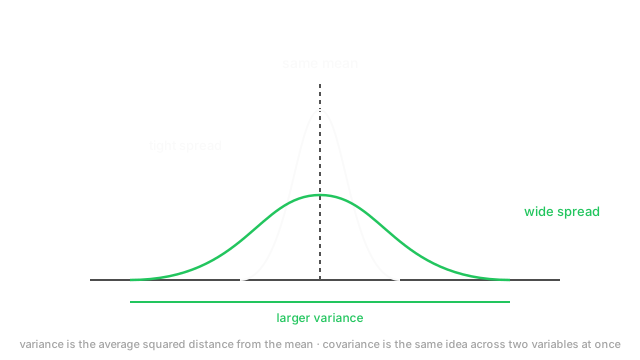
In plain words: take each value's distance from the mean, square it, and average those squares. Squaring does two jobs — it stops positive and negative deviations cancelling, and it penalises far-away points much more than near ones. That second effect is why variance is sensitive to outliers.

Squaring leaves variance in squared units, which is awkward: the variance of a time in minutes is in minutes-squared. Take the square root and you get the standard deviation $\sigma$ , back in the original units and directly comparable to the mean.

Covariance is the same construction across two variables:

\text{Cov}(X, Y) = E\big[(X - E[X])(Y - E[Y])\big]

In plain words: when both variables are above their means at the same time, the product is positive; when they move oppositely, it is negative; and averaging those products tells you which tendency wins. Notice $\text{Cov}(X, X)$ is exactly $\text{Var}(X)$ — variance is the special case of a variable covarying with itself.

Covariance has no scale, so use correlation

Covariance is unbounded and its size depends entirely on units. Measure a length in metres and then in millimetres, and the covariance changes by a factor of a thousand while the relationship is identical. So a covariance of 4.2 means nothing on its own.

Dividing out both standard deviations fixes it:

\rho = \frac{\text{Cov}(X, Y)}{\sigma_X \, \sigma_Y}

That is the correlation coefficient, and it always lands in $[-1, 1]$ : $+1$ is a perfect straight-line increase, $-1$ a perfect decrease, 0 no linear relationship.

The word linear is load-bearing. Correlation only detects straight-line association. $Y = X^2$ over a symmetric range around zero has a correlation of exactly 0 while being perfectly determined by $X$ . A zero correlation is not evidence of independence, and treating it as such is how people convince themselves a genuinely predictive feature is useless.

Worked example

Take eight values: $[2, 4, 4, 4, 5, 5, 7, 9]$ .

The mean is $40 / 8 = 5$ . The deviations from it are $[-3, -1, -1, -1, 0, 0, 2, 4]$ , and their squares are $[9, 1, 1, 1, 0, 0, 4, 16]$ , which total 32. So:

\text{Var}(X) = \frac{32}{8} = 4, \qquad \sigma = \sqrt{4} = 2

In plain words: values sit about 2 units from the mean on average. Sanity-check that against the data — most points are within 2 of 5, and the 9 is the outlier pulling the number up.

Now covariance. Take $x = [1, 2, 3, 4]$ and $y = [2, 4, 6, 8]$ , so $y$ is exactly $2x$ .

Means are 2.5 and 5. Deviations are $[-1.5, -0.5, 0.5, 1.5]$ and $[-3, -1, 1, 3]$ . Their products are $[4.5, 0.5, 0.5, 4.5]$ , totalling 10, so $\text{Cov} = 10/4 = 2.5$ .

For the correlation, $\text{Var}(x) = 5/4 = 1.25$ and $\text{Var}(y) = 20/4 = 5$ , giving:

\rho = \frac{2.5}{\sqrt{1.25} \times \sqrt{5}} = \frac{2.5}{2.5} = 1

Exactly 1, as it must be for a perfect straight line. The covariance of 2.5 told you the direction; only the correlation told you it was perfect.

Show Me the Code

1import numpy as np2
3x = np.array([2.0, 4, 4, 4, 5, 5, 7, 9])   # shape (8,)4print(x.mean(), x.var(), x.std())           # -> 5.0 4.0 2.0   (ddof=0, population)5print(x.var(ddof=1))                        # -> 4.571...      (ddof=1, sample)6
7a = np.array([1.0, 2, 3, 4])8b = 2 * a                                   # a perfect linear relationship9print(np.cov(a, b, bias=True)[0, 1])        # -> 2.5   population covariance10print(np.corrcoef(a, b)[0, 1])              # -> 1.011
12# The one-pass formula E[x^2] - E[x]^2 collapses when the mean is large.13big = np.array([1e9 + 4, 1e9 + 7, 1e9 + 13], dtype=np.float64)14print((big**2).mean() - big.mean() ** 2)    # -> a wrong, possibly negative number15print(big.var())                            # -> 13.555...  correct

Four and two, matching the hand calculation. The ddof line and the last two lines are each a separate trap, and they are what the next section is about.

Watch Out For

The one-pass variance formula losing all its precision

Algebra says $\text{Var}(X) = E[X^2] - (E[X])^2$ , and it is tempting because it needs one pass and two running totals instead of two passes.

On real data it disintegrates. With values around $10^9$ , $E[X^2]$ is around $10^{18}$ — and float64 carries roughly 16 significant digits, so a variance of 13 has to emerge as the difference between two numbers that agree in their first sixteen digits. Every meaningful digit is destroyed by the subtraction. The result is garbage, and frequently negative, which is impossible for a quantity defined as an average of squares.

This is catastrophic cancellation, and it is not an edge case. Timestamps, sensor readings with an offset, prices in minor units, and any feature you forgot to centre all sit in the danger zone. It also silently corrupts running statistics in streaming code, where the one-pass form is most tempting.

Use np.var, or Welford's algorithm if you genuinely need one pass — it tracks the mean and the sum of squared deviations from the running mean, so no large numbers are ever subtracted. If you ever see a negative variance, this is the cause, every time.

Getting the n versus n-1 denominator wrong

There are two variances. Dividing the squared deviations by $n$ gives the population variance: correct when your data is the entire population. Dividing by $n - 1$ gives the sample variance, which corrects for the fact that using the sample's own mean systematically underestimates the spread of the population it came from.

The libraries disagree with each other by default. NumPy's var and std use $n$ (ddof=0). Pandas' .var() and .std() use $n - 1$ . So the same data through two libraries gives two different numbers, and people lose real time to that discrepancy.

With eight points the gap is not subtle: $32/8 = 4$ versus $32/7 \approx 4.571$ , about 14%. At $n = 3$ it is 50%. It stops mattering as $n$ grows, which is why nobody notices on a large dataset and everybody notices on a five-fold cross-validation — exactly where you are computing a standard deviation to decide whether two models genuinely differ. Pick a convention, state it, and use the same one on both sides of any comparison.

The Quick Version

Expectation is the probability-weighted average — the centre of mass. It is linear even for dependent variables.
Variance is the average squared distance from the mean; standard deviation is its square root, back in the original units.
Squaring makes variance sensitive to outliers. That is a property, not a defect.
Covariance asks whether two variables are unusual at the same time. $\text{Cov}(X, X) = \text{Var}(X)$ .
Covariance has arbitrary units, so divide by both standard deviations to get correlation in $[-1, 1]$ .
Correlation only detects linear association. Zero correlation is not independence.
Never compute variance as $E[X^2] - E[X]^2$ — catastrophic cancellation, and it can return a negative number.
NumPy defaults to dividing by $n$ ; pandas defaults to $n - 1$ . The gap is ~14% at $n = 8$ .