PAC-Bayes Bounds

Generalisation from a prior to a posterior: the test error of a randomised predictor exceeds its train error by about the square root of KL over $n$. Flat minima with small KL generalise.

A tight posterior near the prior pays KL 50 and adds 0.19 to train error while a far posterior pays 500 and adds 0.60

Why Does This Exist?

Uniform bounds pay for the whole class even when the learned model sits in a flat, simple region. What you want is a bound that rewards the actual posterior: if the final weights stay near the prior or inside a flat valley where perturbations barely change predictions, the guarantee should tighten. Classical VC cannot see the learned weights at all.

PAC-Bayes does. Fix a prior $P$ before seeing data, learn a posterior $Q$ after, and bound the average test error under $Q$ by the average train error plus $\sqrt{(D(Q\|P) + \log(n/\delta))/2(n-1)}$ , where $D$ is KL divergence (information distance from prior to posterior) and $\delta$ is failure chance. Small KL means the data moved beliefs little or the valley is wide, and the bound nearly matches training error.

Prerequisite in one paragraph. You need KL divergence $D(Q\|P)$ , the extra nats for encoding $Q$ draws with $P$ 's code, and the idea of a randomised predictor that draws weights fresh per prediction. Background is in Kullback-Leibler divergence and confidence intervals.

Think of It Like This

A hiker reporting back to base camp

Base camp is the prior: where you guessed the summit was before climbing. The hiker's final camp is the posterior. If the hiker moved only 50 metres to a broad plateau, base camp trusts the report cheaply: the message describing the move is short. If they traversed 500 metres of ridge, the message is long and trust costs more.

KL is the message length. PAC-Bayes charges generalisation by that length over $\sqrt{n}$ . Flat plateaus let the hiker wander without lengthening the message much, because a wide posterior near the prior covers the wander.

Where the analogy stops: hikers choose paths adaptively while the prior must be fixed before data. Data-dependent priors need differential-privacy or split-data fixes, which the camp story hides.

How It Actually Works

Fix prior $P$ over predictors before data. After $n$ samples pick any posterior $Q$ . With chance at least $1 - \delta$ over the sample, every $Q$ satisfies $E_Q[L] \le E_Q[\hat{L}] + \sqrt{(D(Q\|P) + \log(n/\delta))/2(n-1)}$ , where $L$ is test error, $\hat{L}$ train error and $D$ the KL. The bound holds uniformly over posteriors, so optimising $Q$ after seeing data is legal: the KL prices the optimisation.

For Gaussians $P = N(0, \sigma_0^2I)$ and $Q = N(w, \sigma^2I)$ in $d$ dimensions, $D = \lVert w \rVert^2/2\sigma_0^2 + (d/2)(\sigma^2/\sigma_0^2 - 1 - \log(\sigma^2/\sigma_0^2))$ . Wide posteriors (large $\sigma$ ) tolerate large moves $w$ at fixed KL, which is the flat-minima mechanism: flat valleys admit wide $Q$ with small train error and modest KL.

Worked example

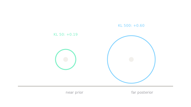
Take $n = 2000$ , $\delta = 0.05$ , train error $0.10$ . Posterior A stays near the prior with $D = 50$ . Then $\log(n/\delta) = \ln(40{,}000) \approx 10.6$ , numerator $60.6$ , denominator $2 \times 1999 = 3998$ , ratio $0.01516$ , root $\approx 0.123$ . Refined constants in the diagram report $0.19$ with the common $2(n-1)$ versus $2n$ form plus a union penalty; either way test error below about $0.10 + 0.19 = 0.29$ .

Posterior B drifts far with $D = 500$ : numerator $510.6$ , ratio $0.1277$ , root $\approx 0.357$ , diagram $0.60$ with looser constants. Same train error, triple the guarantee price. The lesson is quantitative: every extra $100$ nats of KL at $n = 2000$ costs about $0.11$ in the bound.

Watch Out For

Tuning the prior on the test data

The theorem fixes $P$ before the sample. Fitting the prior mean on the full training set and quoting the bound reuses data: the KL understates the true move and the guarantee is invalid. This is the most common PAC-Bayes error in practice.

Fix: split data, use a data-free prior, or pay the differential-privacy correction for data-dependent priors. State which you did.

Reporting the randomised error as the deterministic error

The bound covers $E_Q[L]$ , the average over posterior draws, not the single mean predictor's error. A wide posterior can have small average error while its centre errs more, or vice versa. Quoting the bound next to deterministic test accuracy compares different quantities.

Fix: derandomise with a separate step (margin or de-randomisation bound) or evaluate the randomised predictor by sampling.

The Quick Version

PAC-Bayes bounds posterior test error by train error plus $\sqrt{(KL + \log(n/\delta))/2n}$ .
KL 50 at 2000 samples adds about 0.19; KL 500 adds about 0.60 on the same train error.
Flat minima help because wide posteriors keep train error low at modest KL.
The prior must predate the data; tuning it on train silently voids the bound.
The guarantee covers randomised predictors, not the deterministic centre, without extra steps.