Point Estimation

One dataset, one best guess per unknown. Good guesses center on the truth and tighten as data grows; the page shows how to build and grade them.

Three data points with their mean at 3.67 and deviation brackets showing why dividing by 2 instead of 3 unbiases the variance at 2.33

Why Does This Exist?

Models are built from guesses: the average latency, the conversion rate, the weight vector itself. Each guess compresses a dataset into a single number, and different compressions disagree. The sample mean, the median, a trimmed average, and a model-based estimate all answer the same question differently, so choosing among them needs a grading scheme, not a gut feeling.

Point estimation is that scheme. It defines what an estimator is, grades candidates by bias, variance, and consistency, and supplies default constructions: match the moments, or maximize the likelihood. The likelihood route is maximum likelihood estimation; the summaries underneath are descriptive statistics; the averaging is expectation, variance and covariance.

The one idea you need first

An estimator is a rule for turning data into a guess, like "average the draws," while an estimate is the number it produces on your dataset. Rules have track records across datasets: their bias (systematic off-center) and variance (scatter). Grading the rule, not admiring the number, is the whole discipline.

Think of It Like This

Three archers and their target

One archer clusters arrows tightly but left of center: precise, biased. One scatters widely around the bullseye: unbiased, noisy. One clusters tightly on it: the goal. Judging by a single arrow confuses luck with skill; judging by many exposes each archer's pattern.

Bias is the cluster's off-center, variance is its looseness, and mean squared error is the average squared miss, which splits exactly into bias squared plus variance. More arrows shrink every archer's looseness but never fix the leftward aim: variance yields to data while bias yields only to a better rule. The diagram's deviation brackets are one archer's looseness made visible.

The analogy stops at the target's visibility. Archers see the bullseye, but estimators aim at unknown truths, so bias must be proven mathematically or measured against ground truth, never eyeballed from the cluster alone.

How It Actually Works

For data $X_1, \ldots, X_n$ and a parameter $\theta$ , an estimator $\hat{\theta}$ is graded three ways:

Bias: $E[\hat{\theta}] - \theta$ , the systematic miss. Zero means the rule centers on truth across datasets.
Variance: $\text{Var}(\hat{\theta})$ , the scatter across datasets. Shrinking with $n$ means data helps.
Consistency: convergence to $\theta$ as $n$ grows. The minimum viable promise: infinite data nails it.

In plain words: aim centered, group tightly, and guarantee the group collapses onto truth eventually. Mean squared error combines the first two as $\text{MSE} = \text{bias}^2 + \text{variance}$ , which is why a slightly biased but much tighter rule often wins in practice.

Two default constructions produce candidates. Method of moments equates sample moments to theoretical ones and solves: the mean estimates the distribution mean, the sample variance its variance. Maximum likelihood picks the parameter making the observed data most probable, covered on its own page, and adds optimality guarantees: consistency plus the smallest possible variance at large $n$ .

Worked example

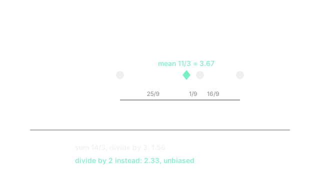
Data $\{2, 4, 5\}$ . The sample mean estimates the center: $\bar{x} = 11/3 \approx 3.67$ .

Variance around it: squared deviations are $(2 - 11/3)^2 = 25/9$ , $(4 - 11/3)^2 = 1/9$ , $(5 - 11/3)^2 = 16/9$ , totaling $42/9 = 14/3$ . The method-of-moments estimator divides by $n = 3$ : $14/9 \approx 1.56$ . But it sits systematically low, because the deviations hug the sample mean rather than the true one. Bessel's correction divides by $n - 1 = 2$ : $7/3 \approx 2.33$ , unbiased. Same data, same deviations, and the divisor decides whether the rule aims centered.

Code

Mean plus both variance flavors on the worked data, with the unbiased correction winning by construction.

1data = [2.0, 4.0, 5.0]2mean = sum(data) / len(data)3biased = sum((v - mean) ** 2 for v in data) / len(data)4unbiased = sum((v - mean) ** 2 for v in data) / (len(data) - 1)5print(round(mean, 4))      # -> 3.66676print(round(biased, 4))    # -> 1.55567print(round(unbiased, 4))  # -> 2.3333

The prints give 3.6667, 1.5556, and 2.3333, matching the hand fractions 11/3, 14/9, and 7/3. The only difference between the last two lines is the divisor, which is the whole lesson.

Watch Out For

Optimizing the estimate instead of the estimator

A number that fits this dataset perfectly, like memorizing every draw, usually estimates terribly: its variance across datasets is enormous. Training error minimized to zero is the same trap at scale. Grade rules by their behavior across datasets, through validation or theory, never by their polish on the data that built them.

Demanding unbiasedness at any variance cost

Unbiased rules can scatter so widely that a slightly biased rule misses less on average: the MSE split says bias squared plus variance, and shrinking variance often pays for small bias handsomely. Regularization buys exactly this trade. Unbiasedness is one virtue, not the verdict.

The Quick Version

An estimator is a rule for guessing; its bias, variance, and consistency grade the rule across datasets.
Mean squared error splits into bias squared plus variance, pricing the classic trade.
Method of moments equates sample and theoretical moments; maximum likelihood maximizes data probability.
On 2, 4 and 5 the mean is 3.67, naive variance 1.56, and Bessel-corrected variance 2.33.
Dividing by n minus 1 instead of n removes the systematic undershoot from fitting the mean first.