Population vs Sample

Why Does This Exist?

Nobody trains on the population. The population is every user, every transaction, every image the model will ever meet, and it is unreachable by definition: meeting all of it would leave nothing to predict. What arrives instead is a sample, a slice of reality that stands in for the whole. Every metric, every fitted parameter, every claimed improvement is computed on the slice and asserted about the whole.

That gap is where statistics lives. Parameters describe populations and stay fixed; statistics describe samples and wobble from sample to sample. Confusing the two turns a lucky slice into a false discovery and a biased slice into a shipped injustice. The summaries themselves are descriptive statistics, the wobble's size is quantified by confidence intervals, and the averaging behind both is expectation, variance and covariance.

The one idea you need first

A parameter is a fixed number describing the population: its mean $\mu$, its variance $\sigma^2$. A statistic is a number computed from a sample: its mean $\bar{x}$, its variance $s^2$. Same formulas, different status. Parameters are the truth; statistics are estimates that dance around it, and the dance has its own distribution.

Think of It Like This

How It Actually Works

Three distinctions carry the whole idea:

• Parameters versus statistics. Greek for the population ($\mu$, $\sigma$), Latin and hats for the sample ($\bar{x}$, $s$). The notation is the reminder: different letters, different epistemic status.
• Sampling variability. Every statistic has a distribution across repeated samples. Its spread shrinks with sample size, roughly as $1/\sqrt{n}$, which is why big samples pin numbers down and small ones swing.
• Bias versus variance of the estimator. An estimator is unbiased when its sampling distribution centers on the parameter. The sample mean is unbiased; the uncorrected sample variance divides by $n$ and sits too low, which is why practice divides by $n - 1$ instead. That correction is Bessel's: one degree of freedom was spent estimating the mean.

In plain words: the population sets the target, the sample takes the shot, and statistics describes the scatter of shots. Good inference picks estimators centered on the target with tight scatter, then reports the scatter honestly.

Worked example

Population $\{4, 6, 8\}$. Parameters: $\mu = 6$ and $\sigma^2 = ((4-6)^2 + 0 + (8-6)^2)/3 = 8/3 \approx 2.67$. Fixed, known, the truth.

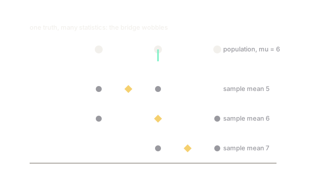
Now draw samples of size 2. Sample $\{4, 8\}$ has mean $6$, exactly the parameter, while sample $\{6, 8\}$ has mean $7$ and $\{4, 6\}$ has mean $5$. One population, three sample means: 5, 6, 7. The wobble is visible with no asymptotics needed.

And the variance trap: sample $\{4, 8\}$ spread around its own mean $6$ gives $((4-6)^2 + (8-6)^2)/2 = 4$ with the naive divisor, above the population's $2.67$, while other samples undershoot. Dividing by $n = 2$ chases the sample's own center; dividing by $n - 1 = 1$ gives $8$, unbiased across samples. Small samples, big corrections.

Watch Out For

The Quick Version

• Populations have fixed parameters; samples yield wobbling statistics that estimate them.
• One tiny population with mean 6 gives sample means of 5, 6, and 7: the wobble is the point.
• Estimator scatter shrinks roughly as one over root n, so big samples pin numbers down.
• Dividing sample variance by n minus 1 instead of n removes the systematic undershoot.
• Convenient slices describe the wrong population exactly; randomness of the ladle matters more than its size.

What to Read Next

• Descriptive Statistics
• Confidence Intervals
• Expectation, Variance and Covariance