Quadratic Programming

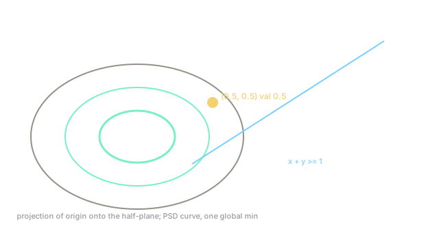
Quadratic cost over straight walls bends the bowls into ellipses. The answer is a projection: the closest feasible point to the free minimum.

Circular contours of x squared plus y squared touch the half-plane x plus y above 1 at the projection (0.5, 0.5)

Why Does This Exist?

Least squares wants the closest fit; portfolios want the lowest variance; SVMs want the widest margin. All three minimize a quadratic over linear walls. LP cannot bend, so it cannot trade smoothly between objectives; QP bends exactly once and stays convex when its matrix is positive semidefinite.

Form: minimize $\\tfrac{1}{2}x^\\top Q x + c^\\top x$ over $Ax \\leq b$ , $Ex = d$ , with $Q \\succeq 0$ . KKT becomes a mixed complementarity system solved by active-set or interior-point methods. It follows linear programming as the curved sibling inside convex optimization.

The one idea you need first

$Q \\succeq 0$ means $x^\\top Qx \\geq 0$ everywhere: bowls, never saddles. Then any KKT point is global. Indefinite $Q$ makes QP NP-hard; the PSD assumption is the whole tractability story.

Think of It Like This

A ball on a tilted elliptical bowl inside a fence

Roll a ball in an elliptical bowl parked inside a straight fence. Free, it settles at the bowl's bottom. Fenced, it settles at the closest fence point to that bottom, pressed against the active rail.

The contact point is the projection under the bowl's metric. Where it stops: real fences have corners that trap balls ambiguously, which is why active-set methods track exactly which rails touch.

How It Actually Works

Unconstrained: solve $Qx = -c$ . Constrained: KKT with $Qx + c + A^\\top\\lambda + E^\\top\\nu = 0$ plus feasibility, $\\lambda \\geq 0$ , slackness. Active-set guesses the touching walls, solves equality QP, updates the guess; interior-point smooths slackness with a barrier. SVM duals, Markowitz portfolios, and MPC controllers are all convex QPs under the hood.

Worked example

Minimize $x^2 + y^2$ subject to $x + y \\geq 1$ . Unconstrained min $(0,0)$ violates. Symmetry says $x = y$ ; constraint gives $x = y = 0.5$ , value $0.25 + 0.25 = 0.5$ . KKT: $2x - \\lambda = 0$ , $2y - \\lambda = 0$ (wall $1 - x - y \\leq 0$ priced $\\lambda$ ): at halves, $\\lambda = 1 \\geq 0$ , slackness $1(1-1) = 0$ . Certified projection with distance $\\sqrt{0.5} \\approx 0.707$ .

Code

1import numpy as np2
3# Project origin onto x + y = 1 by symmetry + check4x = y = 0.55print(round(x**2 + y**2, 2))  # -> 0.56print(round(float(np.sqrt(x**2 + y**2)), 3))  # -> 0.707

Value 0.5 at distance 0.707. Any feasible $(x, 1-x)$ gives $x^2 + (1-x)^2 \\geq 0.5$ with equality at halves.

Watch Out For

Solving with indefinite Q as if convex

Factorization succeeds formally on indefinite $Q$ and returns a saddle or local max certified by nothing. Portfolio "optima" with negative variance directions are the classic casualty.

Check smallest eigenvalue of $Q$ before solving. If negative, convexify, regularize, or switch to global methods.

Warm-starting active set across big changes

Active-set methods fly on small sequential QPs (MPC steps) and crawl when the active set churns completely. Reusing stale wall guesses across regime changes wastes more pivots than cold starts.

Track active-set churn; restart or switch to interior-point when it spikes. If iterations tripled after a model change, the warm start is cold comfort.

The Quick Version

Convex QP needs $Q \\succeq 0$ ; then KKT points are global projections.
$x^2+y^2$ over $x+y \\geq 1$ lands at $(0.5,0.5)$ with value 0.5.
Active-set tracks touching walls; interior-point smooths them.
SVMs, portfolios, and MPC are convex QPs in disguise.
Indefinite $Q$ voids everything; check eigenvalues first.
Warm starts help sequential solves, hurt regime changes.