Linear Programming

Straight-line costs over straight-line walls always corner the answer. The optimum sits at a vertex, so solvers hop corners instead of searching.

Level lines of 3x plus 2y slide until the last feasible touch lands on the vertex at (2, 2) worth 10

Why Does This Exist?

Diets, routes, schedules, and ad splits all ask for the cheapest mix under linear limits: calories above a floor, trucks below capacity, hours within shifts. Nonlinear machinery is overkill; the geometry is polygons and the answer is always a corner.

LP standardizes it: maximize $c^\\top x$ over $Ax \\leq b, x \\geq 0$ . Vertices (basic feasible solutions) hold all optima; simplex walks them, interior-point cuts through. Duality prices resources as shadow prices. It is the linear base of convex optimization solved with the linear tools in linear systems and least squares.

The one idea you need first

Feasible points form a polytope: an intersection of half-spaces. Level sets of $c^\\top x$ are parallel hyperplanes. Sliding the hyperplane until it last touches the polytope lands on a face, generically one vertex.

Think of It Like This

Pushing a ruler across a fenced yard

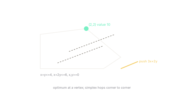
Fences mark the feasible yard. A ruler is one profit level; pushing it uphill keeps profit constant along its edge. The last touch before leaving the yard is usually a single fence post: the vertex.

Ties touch a whole fence segment (multiple optima). Where it stops: real yards have curved or integer fences. Curves need QP/SOCP; integer posts need branch-and-bound, not pushing.

How It Actually Works

Simplex hops vertices via pivots, exponential in the worst case but fast in practice; interior-point follows the central path in polynomial time and wins huge sparse cases. Dual $\\min b^\\top y$ over $A^\\top y \\geq c, y \\geq 0$ prices constraints: $y_i^\\star$ is the marginal value of resource $i$ . Complementary slackness pairs positive prices with tight walls.

Worked example

Maximize $3x + 2y$ subject to $x + y \\leq 4$ , $x + 2y \\leq 6$ , $x, y \\geq 0$ . Vertices: $(0,0) \\to 0$ ; $(4,0) \\to 12$ ; intersection of both lines: subtract to get $y = 2$ , then $x = 2$ , value $3(2)+2(2) = 10$ ; $(0,3) \\to 6$ . Wait: $(4,0)$ gives 12, beating $(2,2)$ : the true optimum is $(4,0)$ with 12. Check feasibility: $4 + 0 = 4 \\leq 4$ , $4 + 0 = 4 \\leq 6$ . Yes. So the vertex $(4,0)$ wins at 12; $(2,2)$ at 10 is the kink where both walls bind but not the top. That correction is the lesson: enumerate all vertices, not just double-tight ones.

Code

1import itertools2
3verts = [(0, 0), (4, 0), (2, 2), (0, 3)]  # enumerated corners4best = max(verts, key=lambda v: 3 * v[0] + 2 * v[1])5print(best, 3 * best[0] + 2 * best[1])  # -> (4, 0) 12

Enumeration picks $(4,0)$ at 12 over $(2,2)$ at 10. Small LPs verify by corners before trusting intuition.

Watch Out For

Rounding LP answers for integer needs

Trucks and people are integers; LP gives 4.7 trucks. Rounding down wastes capacity, rounding up breaks the wall, and the true integer optimum can sit far from the rounded vertex.

Solve the integer program (MILP) for discrete choices. Use LP as the relaxation bound, never the shipment plan.

Declaring unbounded from bad scaling

Missing bounds or huge coefficient ranges make solvers report unbounded or infeasible on feasible models. A forgotten $x \\leq$ cap lets profit run to infinity along a ray.

Bound variables sanely and scale coefficients near 1. If unbounded, ask which ray escapes and whether it is real or a missing wall.

The Quick Version

Linear cost over a polytope optimizes at a vertex; enumerate or hop corners.
Example peaks at $(4,0)$ with 12, beating double-tight $(2,2)$ at 10.
Simplex walks vertices; interior-point cuts through for huge sparse cases.
Dual variables are shadow prices of resources; slackness pairs them with tight walls.
Integer needs MILP, not rounded LP.
Scale and bound models before trusting unbounded verdicts.