Randomized SVD

Find a huge matrix's top directions with randomness: sketch it down to a thin sample, solve the small problem, lift the answer back up.

A tall thin random sketch compresses the giant matrix to a small core, the small SVD solves the core, and lifting back recovers the top directions

Why Does This Exist?

Truncated SVD on a million by million matrix costs $O(n^3)$ and materializes dense factors that dwarf memory. Yet the goal is only the top $k$ directions, and randomness finds them cheaply. Randomized SVD multiplies $A$ by a thin random sketch $\Omega$ with $k + 10$ columns, orthogonalizes the sample $Y = A\Omega$ into $Q$ , compresses to the small core $B = Q^\top A$ , and decomposes $B$ instead. Cost drops to sketch plus small solve, and the error sits within a small factor of the optimal rank $k$ error with overwhelming probability.

That powers PCA on data that never fits in RAM, fast LSA on term document matrices, and near real time recommender updates. Exact foundations are in singular value decomposition. The compression payoff is in PCA derivation.

The one idea you need first

A random projection preserves geometry. $Y = A\Omega$ captures the range of the top directions because random vectors have components along everything, amplified where $A$ stretches most. Oversampling by a few extra columns beyond $k$ plus one or two power iterations with $AA^\top$ sharpens the capture on flat spectra.

Think of It Like This

Polling instead of a census

A census interviews everyone at enormous cost. A poll interviews a random sample and estimates the totals within a known margin of error. Nobody confuses the poll with the census, but decisions run on polls because the error bars suffice.

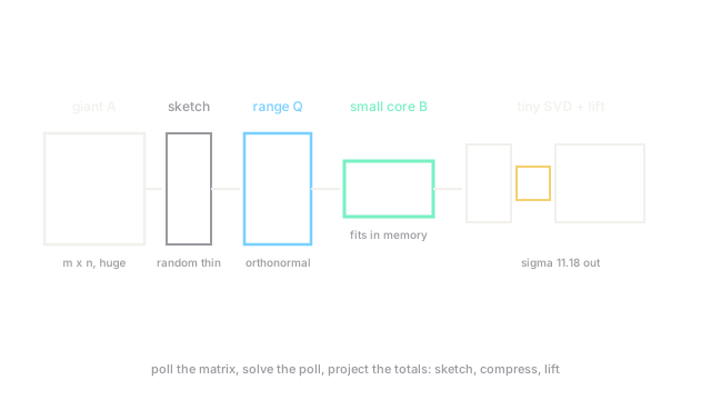
Randomized SVD polls a matrix. The sketch $\Omega$ is the random sample of directions. The small core $B$ is the tabulated poll. The lifted factors are the projected totals. Oversampling is polling extra respondents in volatile districts. Power iterations are callback rounds that sharpen fuzzy answers.

Where it stops: polls need a sampling frame that reaches everyone, and matrices need a sketch that reaches the top range. A sketch too thin for a flat spectrum misses like a poll that skips a whole district.

How It Actually Works

Four stages for target rank $k$ with oversampling $p$ :

Sketch. Draw Gaussian $\Omega$ with shape $n \times (k+p)$ and form $Y = A\Omega$ . Optionally sharpen with $q = 1$ or $2$ steps of $Y = (AA^\top)^q A\Omega$ .
Orthogonalize. Thin QR gives $Y = QR$ . The columns of $Q$ span the sampled range.
Compress. Form $B = Q^\top A$ with shape $(k+p) \times n$ . The giant problem now fits in memory.
Solve small. Take the SVD $B = \tilde{U}\Sigma V^\top$ and lift $U = Q\tilde{U}$ . Truncate to $k$ .

Error sits within $(1 + \epsilon)$ of optimal with probability $1 - \delta$ , where oversampling and power iterations trade cost against both. Fixed seeds make it reproducible. Without them, two runs return different but equally valid bases.

Worked example

Approximate the rank one matrix $A = \begin{bmatrix} 3 & 4 \\ 6 & 8 \end{bmatrix}$ . Its Gram matrix is $A^\top A = \begin{bmatrix} 45 & 60 \\ 60 & 80 \end{bmatrix}$ with trace $125$ and determinant $45 \times 80 - 60 \times 60 = 3600 - 3600 = 0$ , so the eigenvalues are $125$ and $0$ and the singular values are $\sqrt{125} \approx 11.1803$ and $0$ .

Sketch with the deterministic one column $\Omega = [1, 0]^\top$ :

Y = A\Omega = \begin{bmatrix} 3 \\ 6 \end{bmatrix}

One column captures the entire range because the matrix is rank one. Normalize to $Q = [1, 2]^\top / \sqrt{5}$ . Compress to $B = Q^\top A = [15/\sqrt{5}, 20/\sqrt{5}] = [3\sqrt{5}, 4\sqrt{5}]$ . Its norm is $\sqrt{45 + 80} = \sqrt{125} \approx 11.1803$ . The sketch route recovers $\sigma_1$ exactly, with zero dense $m \times n$ factor ever formed.

Code

The point is the check: confirm the sketched singular value matches the exact one.

1import numpy as np2
3
4A = np.array([[3.0, 4.0], [6.0, 8.0]])5exact = np.linalg.svd(A, compute_uv=False)6Y = A @ np.array([[1.0], [0.0]])  # one-column sketch7Q, _ = np.linalg.qr(Y)8B = Q.T @ A9sketched = np.linalg.svd(B, compute_uv=False)10print([round(float(v), 4) for v in exact])  # -> [11.1803, 0.0]11print(round(float(sketched[0]), 4))  # -> 11.1803

Watch Out For

Skimping on oversampling with a flat spectrum

When the top singular values decay slowly, a tight sketch with $p = 0$ mixes the $k$ -th direction with the tail and the truncation wobbles between runs. Oversample by $5$ to $10$ and add one power iteration. Both are cheap insurance, and the error bounds assume you bought it. Flat spectra are exactly where naive sketches embarrass.

Leaving the sketch unseeded in a pipeline

Unseeded randomness returns a different valid basis every run. Components flip, signs change, downstream caches invalidate, and tests flake. Seed the generator and log the seed with the artifacts. Randomized does not have to mean irreproducible.

The Quick Version

Randomized SVD sketches $Y = A\Omega$ , orthogonalizes to $Q$ , solves small $B = Q^\top A$ , and lifts back.
The rank one demo recovers $\sigma_1 = 11.1803$ through a single sketch column.
Cost falls from $O(n^3)$ to sketch plus small solve, with near optimal error at high probability.
Oversample $5$ to $10$ and power iterate once on flat spectra.
Seed every sketch. Different valid bases per run break caches and tests.