Sinkhorn Algorithm

Sinkhorn solves entropy-smoothed transport by alternately rescaling matrix rows and columns, giving fast GPU-friendly approximate couplings.

Alternate row and column scalings converge a kernel to the required margins

Why Does This Exist?

Exact OT linear programs scale cubically and resist GPUs. Adding a little entropy turns the problem into matrix scaling with a unique solution reachable by alternating normalization: divide rows to hit source margins, divide columns to hit target margins, repeat. Each step is a batched multiply, so thousands of transport problems solve in parallel on accelerators.

It is the default OT solver in ML pipelines. Theory: entropic regularization. Primal: Monge and Kantorovich.

The one idea you need first

The Gibbs kernel $K_{ij} = \exp(-C_{ij}/\epsilon)$ turns costs into affinities: cheap routes get weight near 1, expensive ones near 0. The optimal coupling has factored form $\pi = \text{diag}(u)K\text{diag}(v)$ .

Think of It Like This

Balancing a spreadsheet two ways

A budget table must hit row totals and column totals at once. Fix the rows and columns break; fix the columns and rows break. So you alternate: scale each row to its target, then each column, then rows again.

Each pass halves the remaining error and the table settles on the unique sheet satisfying both. Sinkhorn is that alternating fix with multiplicative instead of additive corrections.

Where the analogy stops: the kernel encodes costs exponentially, so tiny regularization makes entries underflow without log-domain care.

How It Actually Works

Iterate $u \gets \mu/(Kv)$ , $v \gets \nu/(K^Tu)$ from $v = 1$ . Each sweep is $O(nm)$ . Convergence is linear with rate tied to the kernel's contraction; small $\epsilon$ sharpens the plan but slows and destabilizes iterations. Log-domain (softmin updates on potentials $f, g$ ) fixes underflow.

Worked example

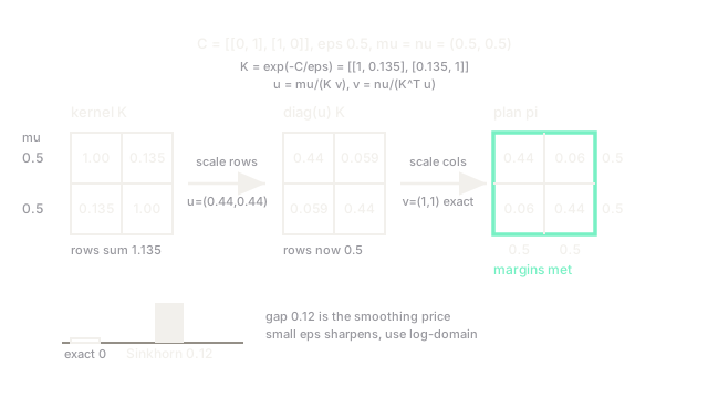
$\mu = \nu = (0.5, 0.5)$ , $C = [[0,1],[1,0]]$ , $\epsilon = 0.5$ : $K = [[1, e^{-2}],[e^{-2},1]] \approx [[1, 0.135],[0.135,1]]$ :

Init $v = (1,1)$ : $Kv = (1.135, 1.135)$ . $u = (0.440, 0.440)$ .
$K^Tu = (0.5, 0.5)$ . $v = (1.0, 1.0)$ . Already converged in one step by symmetry.
Plan $\pi_{ij} = u_i K_{ij} v_j$ : diagonal $0.44$ , off-diagonal $0.06$ . Cost $2 \times 0.06 \times 1 = 0.12$ plus entropy smoothing. Exact LP would put $0.5$ on the diagonal with cost $0$ . The $0.12$ gap is the smoothing price at $\epsilon = 0.5$ .

Code

1import numpy as np2
3
4def sinkhorn(mu: np.ndarray, nu: np.ndarray, C: np.ndarray, eps: float, iters: int = 100) -> np.ndarray:5    K = np.exp(-C / eps)  # Gibbs kernel from costs6    v = np.ones_like(nu)7    for _ in range(iters):8        u = mu / (K @ v)      # match row margins9        v = nu / (K.T @ u)    # match column margins10    return np.diag(u) @ K @ np.diag(v)11
12
13C = np.array([[0.0, 1.0], [1.0, 0.0]])14print(np.round(sinkhorn(np.array([0.5, 0.5]), np.array([0.5, 0.5]), C, 0.5), 3))15# -> [[0.44 0.06] [0.06 0.44]] matching the hand computation

Watch Out For

Running Sinkhorn in raw space with tiny epsilon

Entries $\exp(-C/\epsilon)$ underflow to zero below about $10^{-38}$ in float32, producing division by zero and NaN plans. Small $\epsilon$ triggers it first.

Switch to log-domain softmin updates or stabilize with periodic rescaling once $\epsilon$ drops under the cost median.

Stopping after a fixed 10 iterations always

Loose tolerance leaves margin errors that downstream barycenters amplify into visible artifacts. Fixed counts ignore problem difficulty.

Check marginal violation $\|r - \mu\|_1$ and iterate to $10^{-6}$ or your loss tolerance.

The Quick Version

Sinkhorn solves entropic OT by alternating row and column rescaling.
The Gibbs kernel encodes costs; scaling vectors enforce margins.
Each iteration is matrix-vector products, hence GPU friendly.
Small regularization sharpens plans but needs log-domain arithmetic.
Verify marginal errors instead of trusting fixed iteration counts.