Stability Analysis

Deciding whether nearby motion returns, escapes, or splits: linearize at the equilibrium and let the eigenvalues vote.

Arrows on a line point back toward the stable point 2 from both sides while a saddle sketch splits in one direction and attracts in the other

Why Does This Exist?

Every trained model, controller, and simulation rests at some equilibrium (a minimum, a setpoint, a steady state), and the question is never just where it sits but what happens when kicked. Stable means returns, asymptotically stable means returns and stays, unstable means escapes, and saddles attract along some directions while ejecting along others. Getting this wrong ships controllers that oscillate, optimizers that diverge, and simulations that "converge" to a repeller because the stepper damped the escape. Linearization plus Lyapunov is the standard verdict; the certificate machinery is in Lyapunov analysis and the eigen-machinery in eigenvalues.

The one idea you need first

At equilibrium $f(x^*) = 0$ , the Jacobian $Df(x^*)$ governs nearby motion: $\dot{y} \approx Df(x^*)y$ for displacement $y$ . Negative real parts pull back, positive push away, and mixed signs split into stable and unstable manifolds.

Think of It Like This

Bowls, hills, and passes

A ball in a bowl returns when nudged: stable, and with friction it settles (asymptotically stable). A ball balanced on a hilltop flees: unstable. A ball at a mountain pass rolls back along the ridge but away down the valley: a saddle, stable in one direction and unstable in another.

The bowl's steepness sets the return speed (eigenvalue magnitude), and a flat mesa (zero eigenvalue) refuses to vote: the ball may drift, stick, or creep depending on finer shape, which is exactly where linearization goes silent and nonlinear analysis takes over.

Where the analogy stops: real state spaces have spirals (complex pairs), limit cycles, and basins with fractal edges that no hillside shows.

How It Actually Works

One dimension. $\dot{x} = f(x)$ at $f(x^*) = 0$ : stable if $f'(x^*) < 0$ (arrows point inward), unstable if $> 0$ . Rate $|f'|$ sets the exponential time constant.

Higher dimensions. Eigenvalues $\lambda$ of $Df(x^*)$ : all $\mathrm{Re}(\lambda) < 0$ means asymptotically stable; any $\mathrm{Re}(\lambda) > 0$ means unstable; mixed means saddle with stable manifold along the negative eigenvectors. Complex pairs $\alpha \pm i\beta$ spiral with decay $\alpha$ and frequency $\beta$ .

Beyond linearization. Zero real parts need center-manifold or Lyapunov functions; global claims need basins, not just local arrows. Hartman-Grobman justifies the linear picture near hyperbolic equilibria (no zero real parts).

Worked example

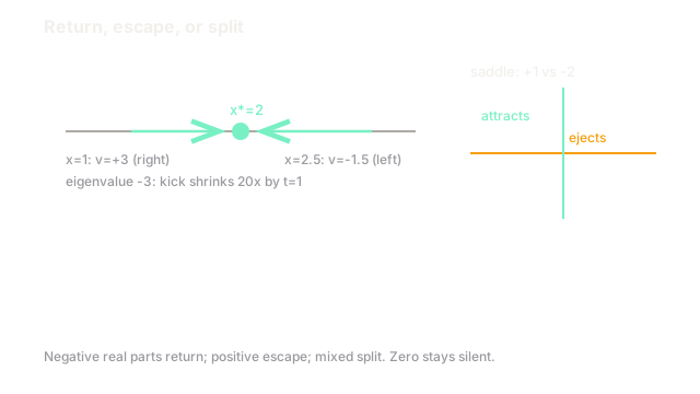
$\dot{x} = -3x + 6$ . Equilibrium where $-3x + 6 = 0$ : $x^* = 2$ . Derivative $f' = -3 < 0$ : stable with rate $3$ .

Kick to $x = 2.5$ : velocity $\dot{x} = -3(2.5) + 6 = -7.5 + 6 = -1.5$ , pointing left back toward $2$ . Kick to $x = 1.0$ : $\dot{x} = -3 + 6 = 3$ , pointing right back toward $2$ . Solution $x(t) = 2 + (x_0 - 2)e^{-3t}$ : a $0.5$ displacement shrinks to $0.5e^{-3} \approx 0.025$ by $t = 1$ , twenty-fold in one unit of time.

Contrast the saddle $\dot{x} = x$ , $\dot{y} = -2y$ : eigenvalues $1$ and $-2$ . The $y$ -axis attracts ( $e^{-2t}$ ) while the $x$ -axis ejects ( $e^{t}$ ): typical starts swing in along $y$ then exit along $x$ .

Watch Out For

Trusting linearization at zero eigenvalues

When the leading eigenvalue sits at zero, the linear picture is a flat vote: stability is decided by higher-order terms, and both fates (and slow drift) occur with identical linearizations. Pitchfork and Hopf bifurcations live exactly here.

Symptom: linear analysis says "marginally stable" while simulations variously stick, drift, or oscillate depending on step and noise. Fix: run center-manifold reduction or construct a Lyapunov function, and treat zero-real-part verdicts as "unknown, analyze further" rather than "stable".

Reading solver damping as ODE stability

Implicit steppers damp fast modes by construction: a stiff unstable mode can look settled because the method killed it, not because the ODE attracts. Conversely, an explicit stepper can oscillate on a calm stable problem past its stability boundary.

Symptom: refining the step flips stable to unstable or vice versa. Fix: separate the two stabilities (test the ODE with tight tolerances and the method against known stability regions), and never certify an equilibrium from one discretization at one step.

The Quick Version

Linearize at $f(x^*) = 0$ ; Jacobian eigenvalues vote: negative returns, positive escapes, mixed splits.
The worked point 2 with eigenvalue $-3$ pulls a 0.5 kick down to 0.025 by $t = 1$ .
Saddles attract along stable eigenvectors and eject along unstable ones.
Zero real parts need nonlinear tools; linearization stays silent there.
Discretization has its own stability: verify against refinement, not one run.