Stationary Distributions

The long-run share of time a Markov chain spends in each state. Start it anywhere and the visit fractions settle onto one fixed vector.

A two-state chain with flip rates 0.2 and 0.3 settles so that 60 percent of long-run visits land on state A and 40 percent on state B

Why Does This Exist?

A Markov chain tells you where you go next, but most questions about it are long-run questions. What fraction of customers sit in each subscription tier after a year of monthly switching? What share of page views lands on each article when readers keep clicking related links? The one-step matrix answers neither directly. The stationary distribution does: it is the row vector $\pi$ that the transition matrix $P$ leaves unchanged, $\pi P = \pi$ .

When it exists and the chain forgets its start, every initial distribution flows toward it. That is why MCMC works: Markov chain Monte Carlo designs a chain whose stationary distribution is the posterior you want, then reads samples off the chain instead of computing the posterior in closed form.

The one idea you need first

A transition matrix $P$ has rows that sum to 1. Entry $P_{ij}$ is the probability of moving from state $i$ to state $j$ in one step. A distribution is a row vector $\pi$ of nonnegative numbers summing to 1. Multiplying $\pi P$ advances the distribution one step. Stationarity means the advance changes nothing. The full treatment of chains is in Markov chains.

Think of It Like This

Two rooms and a restless crowd

A museum has two rooms, A and B. Every minute, 20 percent of the people in A wander into B, and 30 percent of the people in B wander into A. Nobody enters or leaves the building.

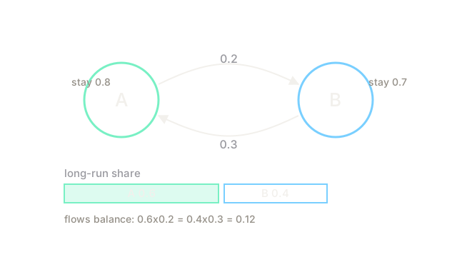
Early on the split swings around, because it depends on where the crowd started. But there is exactly one split that reproduces itself: if 60 percent are in A, then A loses $0.6 \times 0.2 = 0.12$ of the crowd and gains $0.4 \times 0.3 = 0.12$ back from B. Equal flows, frozen split. Start anywhere and the rooms drift to 60/40 and stay there.

Where the analogy stops: real chains can have structure that blocks settling, like a strict two-step cycle or a trap state you never leave. Settling needs the chain to be able to revisit states flexibly, which is what ergodicity pins down.

How It Actually Works

Stationarity is the global balance condition. For every state $j$ :

\pi_j = \sum_i \pi_i P_{ij}

In words: the long-run share of visits to $j$ equals the share arriving from all states, including $j$ itself. Plus the normalization $\sum_j \pi_j = 1$ . For a finite chain these linear equations plus normalization determine $\pi$ whenever the chain has one closed communicating class.

Worked example

Two states, A and B. From A you stay with probability 0.8 and move to B with 0.2. From B you move to A with 0.3 and stay with 0.7:

P = \begin{bmatrix} 0.8 & 0.2 \\ 0.3 & 0.7 \end{bmatrix}

Write $\pi = [\pi_A, \pi_B]$ and impose $\pi P = \pi$ with $\pi_A + \pi_B = 1$ . The first balance equation gives $\pi_A = 0.8\pi_A + 0.3\pi_B$ , so $0.2\pi_A = 0.3\pi_B$ , meaning $\pi_A / \pi_B = 3/2$ . With the sum constraint, $\pi_A = 0.6$ and $\pi_B = 0.4$ . Check: $0.6 \times 0.8 + 0.4 \times 0.3 = 0.48 + 0.12 = 0.6$ . It reproduces itself.

Watch it converge. Start everyone in A, $\pi^{(0)} = [1, 0]$ . Then $\pi^{(1)} = [0.8, 0.2]$ , $\pi^{(2)} = [0.8 \times 0.8 + 0.2 \times 0.3,\ 0.8 \times 0.2 + 0.2 \times 0.7] = [0.70, 0.30]$ , $\pi^{(3)} = [0.65, 0.35]$ . The gap to $[0.6, 0.4]$ halves each step, because the second eigenvalue here is $1 - 0.2 - 0.3 = 0.5$ .

Code

Repeated multiplication is the whole algorithm. This runs power iteration from a cold start and checks the fixed point, which is also the convergence test people use on large chains.

1import numpy as np2
3P = np.array([[0.8, 0.2], [0.3, 0.7]])  # rows sum to 14pi = np.array([1.0, 0.0])  # cold start: everyone in A5for _ in range(20):6    pi = pi @ P  # advance one step7print(np.round(pi, 4))  # -> [0.6 0.4]8print(np.allclose(pi @ P, pi))  # -> True

Twenty steps is overkill on purpose: the error shrinks by a factor of 0.5 per step, so after 20 steps it sits near $10^{-6}$ . On a chain with thousands of states you stop when pi @ P and pi agree to your tolerance, not after a fixed count.

Watch Out For

Assuming every chain has exactly one

A chain with two disconnected halves has infinitely many stationary distributions, one per weighting of the halves. A chain with an absorbing state plus a transient state has $\pi$ concentrated on the absorber, and the transient share is zero no matter how interesting the transient looks. Before solving, check the chain has a single closed class. If your solver returns something that puts zero mass where you expected traffic, the chain structure is usually the explanation, not the solver.

Reading a finite-horizon histogram as the stationary vector

After 50 steps from a cold start, the visit fractions still carry the start. The gap decays like $|\lambda_2|^n$ where $\lambda_2$ is the second-largest eigenvalue magnitude, so a chain with $\lambda_2 = 0.99$ needs thousands of steps, not dozens. Discard a burn-in and compare the first and second halves of the run. If they disagree, you have not converged.

The Quick Version

A stationary distribution satisfies $\pi P = \pi$ : advancing one step changes nothing.
It is the long-run share of visits per state, found from the balance equations plus normalization.
In the worked chain with flip rates 0.2 and 0.3, it is $[0.6, 0.4]$ , and a cold start halves its gap each step.
MCMC works by building a chain whose stationary distribution is the target posterior.
Uniqueness needs one closed communicating class; periodic or disconnected chains break it.
Convergence speed is set by the second eigenvalue, so always discard a burn-in.