Markov Chain Monte Carlo (MCMC)
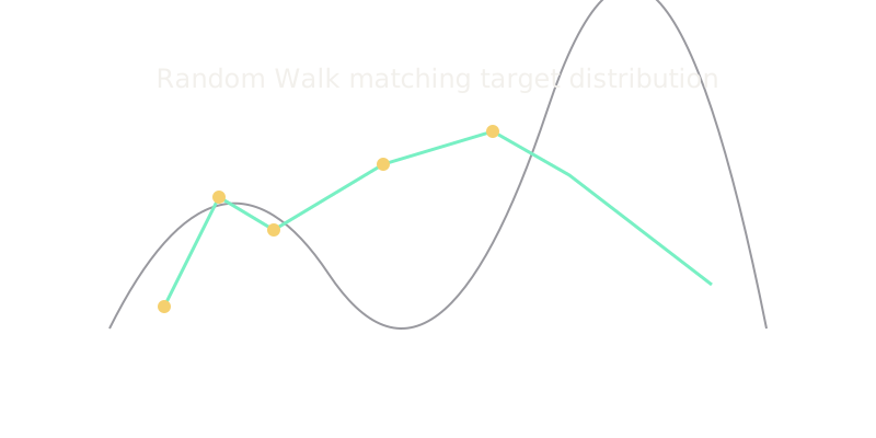
When a distribution is too tangled to sample directly, you wander at random but keep the steps that land in likely places, so where you spend time draws the shape.
Why Does This Exist?
You fit a Bayesian model and want the posterior mean, a credible interval, a prediction average. The posterior has a form you can write down but cannot integrate. It lives in dozens of dimensions, its normalising constant is unknown, and direct sampling is out of reach.
That is the exact gap Monte Carlo methods leave open. Plain Monte Carlo assumes you can already draw from the target. When you cannot, you need a way to turn a rule for wandering around into samples from the right place. MCMC is that bridge.
This page covers the wandering rule and the keep-or-stay decision that makes it work. The chain itself is taught in Markov chains. The posterior setting that motivates most uses is in Bayesian inference. The efficient physics-based sequel is Hamiltonian Monte Carlo.
The one idea you need first
A Markov chain is a sequence where the next state depends only on the current one, through fixed transition probabilities. Given enough steps, many chains settle into a stationary distribution that they then keep sampling. MCMC designs a chain whose stationary distribution equals your target, so running the chain draws from the target. The full treatment is in Markov chains.
Think of It Like This
A census taker who wanders a hilly town
You must estimate where people live in a town built on steep hills, but you have no address list. Your rule is simple. From wherever you stand, pick a nearby house at random and walk toward it. Then compare: if the new street looks busier than your current one, move there. If it looks quieter, still move sometimes, with odds matching how busy it looks relative to where you are.
So a street twice as busy wins every proposal into it, while a street one quarter as busy wins only one proposal in four. Rejections mean you stay put and count your current house again.
Run this for weeks and your notebook maps the town. You spent most nights in dense neighbourhoods and few on empty ridges, not because you planned it but because the keep-or-stay rule steered you. That notebook is your sample.
Where it stops: a real census taker learns the map and plans routes. This walker never learns. Every proposal is as blind as the first, which is why the early wandering must be thrown away.
How It Actually Works
Call the target . You can evaluate an unnormalised version , so ratios equal true ratios because the unknown constant cancels. That cancellation is the whole trick. You never need the constant.
From current state , propose from a proposal . In plain words: is your random step rule, such as adding Gaussian noise. Then accept with probability:
Here is the acceptance probability, is the unnormalised target, and the ratio corrects for asymmetric steps. With a symmetric step such as Gaussian noise, the ratio equals 1 and the rule simplifies to . Moves uphill always win. Moves downhill win in proportion. On rejection you stay at and record it again, which is what keeps the time spent in each region proportional to its mass.
Gibbs sampling as a special case
Gibbs sampling cycles through coordinates and samples each one from its conditional given the rest. Each such move accepts with probability 1, so it is Metropolis-Hastings where the proposal was chosen to make always. Use it when those conditionals have a direct sampler. Otherwise use Metropolis-Hastings.
Worked example
Take a two-place target with and , and a symmetric proposal that always suggests the other place. Only the ratio matters, and you can compute both directions by hand:
- From , propose : ratio , so . You always move.
- From , propose : ratio , so . You move one time in four and stay the other three.
That asymmetry is the sampler. It leaves rarely and returns to always, so a long run spends about 80 percent of its steps at and 20 percent at , matching . Discard the first few dozen steps as burn-in, because the chain starts wherever you dropped it rather than from .
Code
The point is the check: a tiny Metropolis loop on the two-place target should recover 0.8 and 0.2 without ever being told the normalising constant, since only ratios are used.
import random
def run_mcmc(n: int = 20000, seed: int = 0) -> dict[str, int]: random.seed(seed) weights = {"A": 0.2, "B": 0.8} # unnormalised is fine here cur = "A" counts = {"A": 0, "B": 0} for _ in range(n): prop = "B" if cur == "A" else "A" ratio = weights[prop] / weights[cur] # constant cancels if random.random() < min(1.0, ratio): cur = prop counts[cur] += 1 return counts
counts = run_mcmc()print(counts) # -> {'A': 3965, 'B': 16035}print(round(counts["B"] / 20000, 3)) # -> 0.802The 0.802 matches the target 0.8 within sampling noise. Change the seed and the counts wobble but stay near 80 and 20, which is exactly the claim to test.
Watch Out For
Trusting the chain before it has mixed
The first samples reflect your starting point, not the target. Start at an unlikely and the chain needs many steps to wander into the mass. Summaries taken over those early steps inherit the start.
Burn-in is the fix, and it is deletion, not weighting. Drop the first chunk outright, run several chains from spread-out starts, and compare them. If the chains disagree with each other, none of them has mixed and no pooled average is safe.
Tuning the step size by feel and getting sticky chains
A tiny proposal accepts almost always but crawls, so successive samples nearly repeat and averages converge slowly. A huge proposal leaps far but almost always lands somewhere worse and gets rejected, so the chain sits still for long stretches. Both look like sampling and both understate uncertainty.
Watch the acceptance rate and the trace, not just the final histogram. For a simple random-walk Metropolis target, acceptance near 20 to 40 percent in higher dimensions is a sane starting aim. If the trace looks like flat plateaus with rare jumps, shrink the step. If it looks like a slow crawl, grow it.
The Quick Version
- MCMC draws from a distribution you cannot sample directly by running a chain designed to settle on it.
- You only need ratios of an unnormalised target, since the unknown constant cancels.
- Metropolis-Hastings proposes a random step and keeps it with probability . Uphill always wins, downhill wins in proportion.
- On rejection you stay put and count the current state again, which is what allocates time by mass.
- The two-place example gives acceptance 1 one way and 0.25 the other, so a long run spends 80 percent at .
- Gibbs sampling is the special case where each conditional move accepts with probability 1.
- Throw away burn-in, run several chains from different starts, and distrust agreement that you have not checked.