Math

Statistical Power and Sample Size

The probability your test finds a real effect. Work it out before you run the experiment, because a test with low power that returns nothing has not told you the effect is absent — it has told you nothing at all.

$Power is the share of the alternative distribution that falls past the significance threshold, so the two distributions must be far enough apart relative to their width before a real effect can be detected reliably$

Power is the share of the alternative distribution that falls past the significance threshold, so the two distributions must be far enough apart relative to their width before a real effect can be detected reliably

Why Does This Exist?

Because "no significant difference" is the most misread sentence in machine learning evaluation, and power analysis is what tells you whether it meant anything.

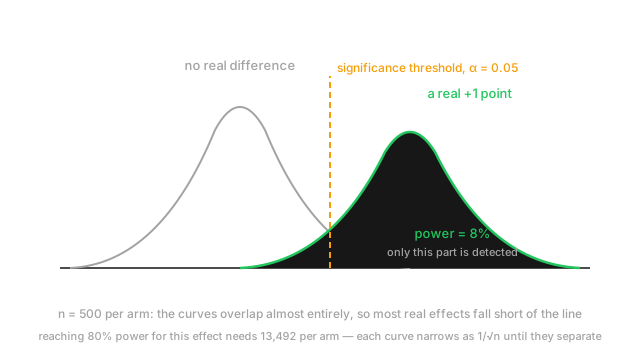
Here is the shape of it. You improve a model, the offline accuracy goes from 90.0% to 91.0%, and you run the comparison on a 500-example test set. The p-value comes back at 0.62. Someone concludes the change does not help and the work is dropped.

But a 500-example test set has roughly 8% power to detect a one-point difference at that accuracy level. Had the improvement been completely real, this test would have missed it 92 times out of 100. The experiment did not fail to find an effect; it was never capable of finding one. Running it was a coin flip weighted heavily toward "no".

That is what an underpowered test buys you: the appearance of evidence with none of the substance. And the mistake is not detectable after the fact from the p-value, which is why the calculation belongs before the experiment.

The consequences are concrete and expensive:

Real improvements get discarded. A team runs ten underpowered comparisons, finds nothing, and concludes the whole research direction is dead.
A/B tests get stopped on noise. Without a pre-computed sample size there is no principled stopping point, so someone looks daily and stops when the number is pleasing. That practice has a false-positive rate far above the nominal 5%.
The effects that do reach significance are inflated. In a low-power study, only unusually large sample estimates clear the threshold, so every published effect is an overestimate. This is the winner's curse, and it is why a 5% offline gain routinely becomes 0.5% online.
Sprints get planned on impossible experiments. "We will measure this in a week" is a claim about sample size, and it is usually checkable in advance in about a minute.

Think of It Like This

A kitchen scale that reads to the nearest 100 grams

You want to know whether a recipe change made the loaf heavier. You have a scale that rounds to the nearest 100 grams.

The change adds about 20 grams. You weigh both loaves and the scale reads 900 for each. Conclusion: no difference.

That conclusion is worthless, and everyone can see why — the instrument cannot resolve 20 grams. Nothing about the reading tells you the change did nothing. It tells you that you used the wrong scale.

Statistical power is the resolution of your experiment, and sample size is what sets it. A test on 500 examples is a scale that reads to the nearest 100 grams. A test on 15,000 is one that reads to the nearest gram.

Three parts of the analogy carry over exactly:

You can compute the resolution before weighing. The scale's specification is printed on it. Your experiment's resolution is a formula, and it needs only the baseline rate, the significance level and the power you want.

Resolution and effect size are the only things that matter, jointly. A coarse scale detects a large change fine. A fine scale is needed for a small one. Neither number means anything alone — the question is always effect size relative to noise.

A negative result from a coarse instrument is not evidence of absence. It is absence of evidence. The two sound similar and are opposites.

Where the analogy understates the problem: a scale's resolution improves linearly with its price, while an experiment's resolution improves only as $\sqrt{n}$ . Halving the effect you can detect costs four times the data. This is why detecting small effects is so much harder than it feels like it should be, and why a "small tweak" can be genuinely unmeasurable at your traffic level.

How It Actually Works

Hypothesis testing has two error types. Power is about the second one.

Type I error, rate $\alpha$ : declaring an effect that is not there. You choose this, conventionally 0.05.
Type II error, rate $\beta$ : missing an effect that is there.
Power $= 1 - \beta$ : the probability of detecting a real effect of a given size. The conventional target is 0.80.

The asymmetry is worth noticing. Everyone sets $\alpha$ deliberately and almost nobody sets $\beta$ , which means the error rate people actually suffer is the one they never chose. A power of 0.80 means a one in five chance of missing a real effect — and that is the good case, the one you get only by planning for it.

Four quantities are locked together, and fixing any three determines the fourth:

Sample size $n$
Effect size — how big a difference you want to be able to catch
Significance level $\alpha$
Power $1 - \beta$

So there are three useful calculations, and it is worth knowing which one you are doing:

Sample size, before the experiment: given the effect you care about and the power you want, how much data? This is the one to run.
Minimum detectable effect (MDE), when $n$ is fixed by your traffic: given the data you can get, what is the smallest effect you could reliably see? Usually the more honest framing, because sample size is rarely a free choice.
Post-hoc power, after the fact: don't. Computing power from your observed effect is a deterministic function of your p-value and adds no information at all. It is a widely-cited mistake.

The formula, and how to read it

For comparing two means at $\alpha = 0.05$ two-sided and 80% power, the required size per group is

n \approx \frac{2\,(z_{\alpha/2} + z_{\beta})^2}{d^2} = \frac{2(1.96 + 0.84)^2}{d^2} = \frac{15.7}{d^2} \approx \frac{16}{d^2}

where $d$ is Cohen's $d$ — the difference in means divided by the standard deviation. In plain words: the sample size you need is about 16 divided by the squared effect size. Worth memorising; it turns most feasibility questions into mental arithmetic.

For two proportions — the accuracy, click-through or conversion case — the same structure with each group's own variance:

n \approx \frac{(z_{\alpha/2} + z_{\beta})^2 \big[p_1(1 - p_1) + p_2(1 - p_2)\big]}{(p_1 - p_2)^2}

Three things to read straight off these:

The effect size is squared in the denominator. Halving the effect quadruples the data. This is the single most important structural fact here.
Variance is in the numerator. Noisier measurements need more data, proportionally. Reducing variance is therefore just as good as increasing $n$ , and often much cheaper — which is what stratification, variance-reduction adjustments like CUPED, and paired designs are all for.
$\alpha$ and power enter only through $(z_{\alpha/2} + z_\beta)^2$ , which changes slowly. Moving from 80% to 90% power multiplies $n$ by about 1.34; correcting $\alpha$ for ten comparisons multiplies it by about 1.5. Real, but second-order next to effect size.

Paired tests change the arithmetic completely

For ML evaluation specifically there is a large win available, and missing it is the most common practical error on this page.

When you compare two models you usually evaluate them on the same test set. That is a paired design, and pairing removes all the variance caused by some examples simply being harder than others — which is the dominant source of variance in a test set. The right test is not a two-proportion test on the two accuracies; it is McNemar's test on the disagreements.

McNemar's test throws away every example both models got right and every example both got wrong, because those carry no information about which is better. It looks only at the cells where they disagree: $b$ examples where A is right and B is wrong, $c$ where B is right and A is wrong. Under the null those are a coin flip, and the required sample size depends on the disagreement rate, not the accuracy.

The practical effect is large. Two models that agree on 95% of examples need far less data to distinguish than an unpaired calculation suggests, because all the signal is concentrated in the 5% where they differ. Using the unpaired formula on a paired design does not give a wrong answer so much as a wildly pessimistic one, and it is why teams conclude they need 10,000 labels when 1,500 would have done.

Worked example

Take the case from the top of the page: a classifier at 90.0% accuracy against a candidate at 91.0%, unpaired, $\alpha = 0.05$ two-sided, 80% power.

The numerator uses both groups' variances:

p_1(1-p_1) + p_2(1-p_2) = 0.90 \times 0.10 + 0.91 \times 0.09 = 0.0900 + 0.0819 = 0.1719

The denominator is the squared difference, $(0.01)^2 = 0.0001$ . With $(1.96 + 0.84)^2 = 7.85$ :

n \approx \frac{7.85 \times 0.1719}{0.0001} = \frac{1.349}{0.0001} = 13{,}492 \text{ per group}

Thirteen and a half thousand examples per arm, to detect one accuracy point. That is the number the 500-example test was up against, and it explains the 8% power quoted earlier.

Now change only the effect. A five-point improvement, 90% to 95%:

n \approx \frac{7.85\,(0.0900 + 0.0475)}{(0.05)^2} = \frac{7.85 \times 0.1375}{0.0025} = 432 \text{ per group}

432 against 13,492. A five-fold smaller effect needs 31 times more data. The quadratic accounts for 25 of that and the variance term for the rest. Anyone who has been surprised by how much traffic an A/B test needs has met this multiplier.

Run it backwards, which is usually the more useful direction. With a test set of 2,000 examples per arm fixed, what is the smallest gap you could detect at 80% power? Rearranging gives $\delta \approx \sqrt{7.85 \times 0.18 / 2000} = 0.0266$ , so about 2.7 accuracy points. Below that, this test set cannot distinguish the models regardless of how the numbers come out, and the correct report is "this evaluation cannot resolve differences under 2.7 points" rather than "no significant difference".

Finally, the same comparison done properly as a paired test. Suppose the two models disagree on 8% of examples, and of those disagreements the new model is right 57% of the time — a genuine but modest edge. McNemar's test needs roughly

n_{\text{disagreements}} \approx \frac{(1.96 + 0.84)^2}{4(0.57 - 0.5)^2} = \frac{7.85}{4 \times 0.0049} = 400

disagreements, which at an 8% disagreement rate means about 5,000 examples total — not per arm, since both models are scored on the same ones. The unpaired design needed 13,492 per arm, so 26,984 labelled evaluations against 5,000: a 5.4-fold reduction for the same statistical question. Same models, same data, better test.

Show Me the Code

1import numpy as np2from scipy import stats3
4Z_A, Z_B = stats.norm.ppf(0.975), stats.norm.ppf(0.80)   # 1.960 and 0.8425K = (Z_A + Z_B) ** 2                                      # 7.8496
7
8def n_per_group(p1: float, p2: float) -> float:9    """Unpaired two-proportion sample size at alpha=0.05, power=0.80."""10    return K * (p1 * (1 - p1) + p2 * (1 - p2)) / (p1 - p2) ** 211
12
13print(round(n_per_group(0.90, 0.91)))         # -> 13492   one accuracy point14print(round(n_per_group(0.90, 0.95)))         # -> 432     five points, 31x less data15print(round(np.sqrt(K * 0.18 / 2000), 4))     # -> 0.0266  MDE from n=200016
17# The power the 500-example test actually had:18se = np.sqrt(0.90 * 0.10 / 500 + 0.91 * 0.09 / 500)19print(round(float(stats.norm.sf(Z_A - 0.01 / se)), 3))    # -> 0.078  not 0.8020
21print(round(K / (4 * (0.57 - 0.50) ** 2)))    # -> 400   McNemar disagreements needed

Every printed value reproduces the hand calculation. The 0.078 is the sentence at the top of the page as a number: that test would have missed a genuine one-point improvement 92% of the time.

Watch Out For

Peeking at a running test and stopping when it turns significant

Every look at an accumulating result is another chance to cross the threshold by luck, and the false-positive rate compounds with the number of looks.

The arithmetic is unforgiving. A test designed for $\alpha = 0.05$ and checked once has a 5% false-positive rate. Checked five times as data accrues, it is around 14%. Monitored continuously to a fixed horizon, it approaches 100% — a random walk crosses any fixed boundary eventually, so a test with no real effect will always show significance if you watch long enough and stop at the right moment. This is not a small correction; it is the difference between a 5% error rate and a guaranteed one.

The behaviour that produces it is entirely natural: the dashboard updates hourly, the p-value dips below 0.05 on day three, and stopping now saves a week. The estimate you ship is also inflated, because you stopped precisely at a favourable fluctuation.

The fixes, and they are well established:

Fix the sample size in advance and do not look at the outcome until you reach it. Simplest, and what the formulas above are for. Monitoring for breakage is fine and necessary; monitoring the primary metric for a decision is not.
Use a sequential design if you need to stop early. Group sequential boundaries (O'Brien–Fleming, Pocock) or always-valid p-values based on confidence sequences let you look whenever you like and remain correct. The cost is a slightly larger sample size at the planned horizon.
Pre-register the primary metric, the effect size and the horizon. One sentence in the experiment doc removes the whole class of problem, and makes the analysis reviewable.

The related trap: running until you reach significance or until you give up. That asymmetry is the same bias with extra steps.

Counting rows as independent when they are not

Every formula on this page assumes $n$ independent observations. Almost no real ML dataset supplies them, and the failure is silent: your effective sample size is far below your row count, so your confidence intervals are too narrow and your p-values too small.

Where the independence quietly fails:

Multiple rows per user. In an A/B test with 100,000 events from 8,000 users, the unit of randomisation is the user, so $n = 8{,}000$ , not 100,000. Using the event count inflates your effective sample size by 12× and shrinks your standard error by $\sqrt{12} \approx 3.5$ . Cluster-robust standard errors, or aggregating to one row per user before testing, is the fix.
Time series and sessions. Consecutive observations are correlated. A month of daily metrics is nowhere near 30 independent measurements, and treating it as such makes every trend look significant.
Grouped or near-duplicate examples. Multiple frames from the same video, several sentences from the same document, augmented copies of one image. Any of these split across train and test also leaks, which is a separate and worse problem.
Cross-validation folds. The $k$ fold scores are not independent — they share training data — so a paired t-test across folds has an anti-conservative error rate. The standard remedies are corrected resampled t-tests or, better, bootstrapping at the level of the independent unit.

The habit that catches all of these: name the independent unit before you compute anything, and check that your $n$ counts those rather than rows. If a single unit can produce many rows, aggregate first or use a method that models the clustering. When in doubt, bootstrap by resampling whole clusters — it needs no formula and respects the dependence structure automatically.

The Quick Version

Power is the probability of detecting a real effect. The conventional 0.80 still means a one-in-five miss rate.
"No significant difference" from an underpowered test is not evidence of no difference. It is no evidence.
Sample size, effect size, $\alpha$ and power are locked together; fix three and the fourth follows.
For two means, $n \approx 16/d^2$ per group at $\alpha = 0.05$ and 80% power. Worth memorising.
Effect size is squared in the denominator, so halving the detectable effect quadruples the data. Detecting one accuracy point at 90% takes about 13,500 examples per arm; five points takes 432.
Compute the minimum detectable effect when $n$ is fixed, which is most of the time. Never compute post-hoc power from an observed effect.
Model comparisons on a shared test set are paired. Use McNemar's test on disagreements — often a several-fold reduction in the labels needed.
Reducing variance substitutes for increasing $n$ , and is usually cheaper. Pairing, stratification and CUPED all do this.
Peeking inflates the false-positive rate toward 100%. Fix $n$ in advance or use a sequential design.
Count independent units, not rows. Multiple events per user, per session or per document all shrink your effective $n$ .