Strong Law of Large Numbers

Averaging independent repeats of the same gamble washes out the luck. The sample mean does not just probably land near the true average; with full certainty it converges there and stays.

Running averages of die rolls swing early then settle onto 3.5 and remain there as more rolls arrive

Why Does This Exist?

Every Monte Carlo estimate, every A/B test readout, every training loss averaged over batches bets on one claim: more samples means the average locks onto truth. The weak law promises the average is probably close at any large fixed sample size. The strong law promises more: with probability one, the whole path of averages converges and never leaves again.

That pathwise promise is what long-running systems need. A dashboard tracking conversion for months wants eventual permanent settling, not a fresh gamble at each checkpoint. This page states the strong law and shows it on dice. The weak-versus-strong contrast sharpens with the central limit theorem, which quantifies the remaining wobble.

The one idea you need first

Almost sure convergence means the bad event (averages fail to settle on truth) has probability exactly zero. It is stronger than convergence in probability, which lets the failure chance shrink but stay positive at every finite $n$ . Averages are in expectation, variance and covariance.

Think of It Like This

A spinning coin counter that stops arguing

A cashier counts a huge jar of mixed coins by weighing handfuls. Early handfuls disagree wildly: one is all quarters, the next all pennies. But as handfuls accumulate, the running average weight per coin creeps toward the jar's true mix and the arguments between successive averages die down for good.

The weak law says any single late handful is probably representative. The strong law says the sequence of running averages itself goes quiet with certainty. Where it stops: certainty is about the math, not the jar. A biased sampling scoop breaks the identical-distribution assumption and the average settles on the wrong number.

How It Actually Works

Let $X_1, X_2, \ldots$ be independent and identically distributed with $\mathbb{E}|X_1| < \infty$ and mean $\mu = \mathbb{E}[X_1]$ . The strong law (Kolmogorov) says:

\frac{X_1 + \cdots + X_n}{n} \to \mu \quad \text{almost surely}

In plain words: $X_i$ are repeats of one gamble, $\bar{X}_n$ is their running average, and with probability one that average tends to $\mu$ as $n$ grows. Finite absolute mean is the whole price of admission; without it (Cauchy variables) averages never settle. The weak law concludes $\bar{X}_n \to \mu$ in probability under weaker typically stated finite-variance conditions, a strictly weaker promise about each fixed $n$ rather than the path.

Worked example

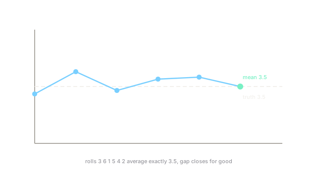
Fair die: $\mu = (1+2+3+4+5+6)/6 = 3.5$ . Roll $3, 6, 1, 5, 4, 2$ . Running averages: $3.0$ , $4.5$ , $10/3 \approx 3.33$ , $15/4 = 3.75$ , $19/5 = 3.8$ , $21/6 = 3.5$ . Sum check: $3+6+1+5+4+2 = 21$ , and $21/6 = 3.5$ exactly.

Early swings ( $\pm 1$ ) dwarf late ones because each new roll carries weight $1/n$ . The strong law says this settling continues: the path locks onto $3.5$ with probability one, and the central limit theorem adds that typical deviations shrink like $1/\sqrt{n}$ .

Code

Running averages of simulated die rolls visibly settle near 3.5 as n grows.

1import numpy as np2
3
4def running_means(rolls: np.ndarray) -> np.ndarray:5    return np.cumsum(rolls) / np.arange(1, rolls.size + 1)  # mean after each roll6
7
8rolls = np.array([3.0, 6.0, 1.0, 5.0, 4.0, 2.0])9print(running_means(rolls))  # -> [3. 4.5 3.33 3.75 3.8 3.5]

Starts at $3.0$ , swings to $4.5$ , lands exactly on $3.5$ : the convergence the theorem guarantees.

Watch Out For

Quoting the law for heavy-tailed data

Symptom: averaging Cauchy-distributed ratios or unbounded losses and watching the mean jump forever. Fix: check $\mathbb{E}|X| < \infty$ first; with infinite mean no law applies and the median is the stabler target.

Reading almost sure as eventually always within epsilon

Symptom: assuming averages cross into an $\epsilon$ -band and freeze there monotonically. Fix: convergence is not monotone; paths can exit and re-enter finitely often. The promise is eventual permanent residence, not a one-way door.

The Quick Version

IID variables with finite mean have sample averages converging to the true mean with probability one.
Almost sure is pathwise and permanent; in-probability is per-checkpoint and weaker.
Six die rolls $3, 6, 1, 5, 4, 2$ average exactly $3.5$ , the fair-die mean.
Each new sample matters like $1/n$ , so early swings fade and late ones barely register.
Infinite-mean variables (Cauchy) never settle; the law simply does not apply.