Basic Concepts in Reinforcement Learning

Why Does This Exist?

In supervised learning, an external supervisor gives an explicit ground-truth label for every input. The model is told immediately what output it should have produced. In unsupervised learning, an algorithm searches for latent structure without any task feedback or external score.

Real-world autonomous intelligence does not fit either regime. When a robotic arm learns manipulation, an autonomous vehicle navigates rush-hour traffic, or an agent plays chess, there is no supervisor standing by to score every micro-action at step 37 of a thousand-step episode. The agent only receives evaluative feedback: occasional positive or negative rewards indicating whether intermediate states and final outcomes were beneficial.

Without the formal framework of Reinforcement Learning (RL), learning by trial and error breaks down in three critical ways:

1. Delayed credit assignment: An action taken early in an episode may produce consequences dozens or hundreds of steps later. Naive optimization cannot tell which past decision caused a delayed success or failure.
2. Distributional shift through action: In static machine learning, the dataset is fixed. In sequential decision-making, every action taken alters the future distribution of states the agent visits. A single mistake moves the agent into unfamiliar regions of the state space.
3. Evaluative vs. instructive feedback: Evaluative feedback tells an agent how well it performed, but not what the optimal action was. The agent must actively explore alternative actions to discover superior strategies.

Reinforcement learning formalizes this interaction into a rigorous mathematical loop where agents learn goal-directed behavior by maximizing long-term cumulative reward.

Think of It Like This

How It Actually Works

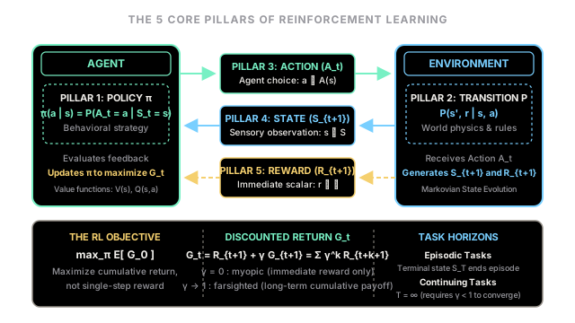
The Five Pillars and the Agent-Environment Loop

At each discrete time step $t = 0, 1, 2, \dots$, the interaction between the agent and the environment proceeds through five interconnected pillars:

The cycle repeats indefinitely or until a terminal state is reached:

1. The agent observes the current state $S_t \in \mathcal{S}$.
2. The agent selects an action $A_t \sim \pi(\cdot \mid S_t)$ according to its policy $\pi$.
3. The environment processes $A_t$, transitions to a new state $S_{t+1} \sim P(\cdot \mid S_t, A_t)$, and emits a scalar reward $R_{t+1}$.
4. The agent receives $S_{t+1}$ and $R_{t+1}$, updating its internal policy or value estimates.

Trajectories, Returns, and the Discount Factor

A sequence of interactions produces an experience trajectory $\tau$:

$\tau = (S_0, A_0, R_1, S_1, A_1, R_2, \dots, S_T)$

Tasks fall into two primary structures:

• Episodic Tasks: Interaction naturally breaks into distinct episodes that terminate at time step $T$ upon reaching an absorbing terminal state (e.g., checkmate, game over, reaching a maze exit).
• Continuing Tasks: Interaction proceeds infinitely without termination ($T = \infty$), such as an automated thermostat, industrial process control, or continuous inventory management.

To evaluate an agent's performance, we do not optimize isolated immediate rewards. Instead, we optimize the cumulative return $G_t$, defined from time step $t$ onward with a discount factor $\gamma \in [0, 1)$:

$G_t = \sum_{k=0}^{\infty} \gamma^k R_{t+k+1} = R_{t+1} + \gamma R_{t+2} + \gamma^2 R_{t+3} + \dots$

This definition yields the fundamental recursive relationship used throughout reinforcement learning:

$G_t = R_{t+1} + \gamma G_{t+1}$

The discount factor $\gamma$ plays two vital roles:

• Mathematical Convergence: When tasks are continuing ($T = \infty$), summing unweighted rewards bounded by $R_{\max}$ would diverge to infinity. When $\gamma < 1$, the geometric series bounds the maximum possible return: $G_t \le \sum_{k=0}^{\infty} \gamma^k R_{\max} = \frac{R_{\max}}{1 - \gamma}$
• Behavioral Horizon: The discount factor tunes the agent's effective planning horizon $H_{\text{eff}} \approx \frac{1}{1 - \gamma}$. When $\gamma = 0$, the agent is purely myopic, maximizing only the immediate reward $R_{t+1}$. As $\gamma \to 1$, the agent becomes farsighted, weighting distant consequences heavily.

Value Functions and the Optimization Target

Because future state transitions and policies can be stochastic, the return $G_t$ is a random variable. An agent evaluates states using expected returns:

• State-Value Function $V^\pi(s)$: The expected return starting from state $s$ under policy $\pi$: $V^\pi(s) = \mathbb{E}_\pi [G_t \mid S_t = s]$
• Action-Value Function $Q^\pi(s, a)$: The expected return of taking action $a$ in state $s$ and thereafter following $\pi$: $Q^\pi(s, a) = \mathbb{E}_\pi [G_t \mid S_t = s, A_t = a]$

The overarching objective of reinforcement learning is to discover an optimal policy $\pi^*$ that maximizes the expected return from the start:

$\pi^* = \arg\max_\pi \mathbb{E}_{\tau \sim \pi} [G_0]$

Worked numerical example

Consider a 4-step episodic trajectory generated by an agent navigating an obstacle course:

$\tau = (S_0, A_0, R_1=+2.0, S_1, A_1, R_2=-1.0, S_2, A_2, R_3=0.0, S_3, A_3, R_4=+10.0, S_4)$

At step 4, the agent reaches the terminal goal state $S_4$. Because $S_4$ is terminal, no subsequent rewards exist, so $G_4 = 0.0$.

Let the discount factor be $\gamma = 0.9$. We compute the return $G_t$ at each step by propagating backwards using $G_t = R_{t+1} + \gamma G_{t+1}$:

1. Terminal step $t = 4$: $G_4 = 0.0$
2. Step $t = 3$: Transition to terminal goal $S_4$ yielding reward $R_4 = +10.0$: $G_3 = R_4 + \gamma G_4 = 10.0 + 0.9 \times 0.0 = 10.0$
3. Step $t = 2$: Transition to intermediate state $S_3$ yielding reward $R_3 = 0.0$: $G_2 = R_3 + \gamma G_3 = 0.0 + 0.9 \times 10.0 = 9.0$
4. Step $t = 1$: Step across rough terrain to $S_2$ yielding penalty $R_2 = -1.0$: $G_1 = R_2 + \gamma G_2 = -1.0 + 0.9 \times 9.0 = -1.0 + 8.1 = 7.1$
5. Initial step $t = 0$: Initial transition from $S_0$ to $S_1$ yielding reward $R_1 = +2.0$: $G_0 = R_1 + \gamma G_1 = 2.0 + 0.9 \times 7.1 = 2.0 + 6.39 = 8.39$

We verify $G_0$ by expanding the full power series directly:

$G_0 = R_1 + \gamma R_2 + \gamma^2 R_3 + \gamma^3 R_4$ $G_0 = 2.0 + 0.9(-1.0) + (0.9)^2(0.0) + (0.9)^3(10.0)$ $G_0 = 2.0 - 0.90 + 0.0 + 0.729 \times 10.0 = 1.10 + 7.29 = 8.39$

Comparing the return at $t=0$ under different values of $\gamma$ illustrates the impact of discounting:

• $\gamma = 0.0$ (myopic): $G_0 = 2.00$ (ignores both the $-1.0$ penalty and the $+10.0$ goal)
• $\gamma = 0.5$ (short-sighted): $G_0 = 2.0 - 0.5 + 0.0 + 1.25 = 2.75$
• $\gamma = 0.9$ (farsighted): $G_0 = 8.39$
• $\gamma = 1.0$ (undiscounted sum): $G_0 = 2.0 - 1.0 + 0.0 + 10.0 = 11.00$

Code

1from dataclasses import dataclass2from typing import List, Sequence3
4@dataclass(frozen=True)5class TransitionStep:6    state: str7    action: str8    reward: float9    next_state: str10
11def compute_discounted_returns(12    rewards: Sequence[float],13    gamma: float14) -> List[float]:15    """Compute backwards cumulative discounted return G_t for each step.16    17    Uses the recursive formulation: G_t = R_{t+1} + gamma * G_{t+1}.18    Runs in O(N) time and O(N) auxiliary space.19    """20    if not (0.0 <= gamma <= 1.0):21        raise ValueError(f"Gamma must be in [0.0, 1.0], got {gamma}")22    23    n = len(rewards)24    returns: List[float] = [0.0] * n25    running_return = 0.026    27    # Backwards accumulation from terminal step T to step 028    for t in reversed(range(n)):29        running_return = rewards[t] + gamma * running_return30        returns[t] = running_return31        32    return returns33
34# Sample episodic trajectory: 4 steps leading to a goal state35trajectory: List[TransitionStep] = [36    TransitionStep(state="S0", action="East",  reward=2.0,  next_state="S1"),37    TransitionStep(state="S1", action="South", reward=-1.0, next_state="S2"),38    TransitionStep(state="S2", action="East",  reward=0.0,  next_state="S3"),39    TransitionStep(state="S3", action="North", reward=10.0, next_state="S4_goal"),40]41
42rewards = [step.reward for step in trajectory]43gammas = [0.0, 0.5, 0.9, 1.0]44
45print("Step-by-step Discounted Returns G_t across Gammas:")46header = f"{'Step':<6} | {'Reward':<8} | " + " | ".join([f"gamma={g:<4}" for g in gammas])47print(header)48print("-" * len(header))49
50all_returns = {g: compute_discounted_returns(rewards, g) for g in gammas}51
52for t, step in enumerate(trajectory):53    ret_str = " | ".join([f"{all_returns[g][t]:<6.2f}" for g in gammas])54    print(f"t={t:<4} | R_{t+1}={step.reward:<4.1f} | {ret_str}")

Expected output:

1Step-by-step Discounted Returns G_t across Gammas:2Step   | Reward   | gamma=0.0  | gamma=0.5  | gamma=0.9  | gamma=1.0 3---------------------------------------------------------------------4t=0    | R_1=2.0  | 2.00   | 2.75   | 8.39   | 11.00 5t=1    | R_2=-1.0 | -1.00  | 1.50   | 7.10   | 9.00  6t=2    | R_3=0.0  | 0.00   | 5.00   | 9.00   | 10.00 7t=3    | R_4=10.0 | 10.00  | 10.00  | 10.00  | 10.00 

Watch Out For

The Quick Version

• Reinforcement learning models sequential decision-making through an agent-environment interaction loop governed by States, Actions, and Rewards.
• The policy $\pi$ determines the agent's behavior, while environment transition dynamics $P(s', r \mid s, a)$ dictate physics, transitions, and feedback.
• The core objective is maximizing expected discounted return $G_t = \sum_{k=0}^{\infty} \gamma^k R_{t+k+1} = R_{t+1} + \gamma G_{t+1}$, rather than picking greedy immediate rewards.
• The discount factor $\gamma \in [0, 1)$ balances short-term survival against long-term planning, and guarantees finite returns in infinite-horizon continuing tasks.

What to Read Next

• Markov Decision Processes
• Value Functions
• Exploration vs. Exploitation