Behavioral Cloning

Instead of designing reward functions, behavioral cloning trains an agent using standard supervised learning to imitate recorded expert demonstrations directly.

Why Does This Exist?

In classic reinforcement learning, defining a reward function that produces the desired behavior without unintended side effects is notoriously difficult. In self-driving vehicles, robotic surgery, and dexterous manipulation, minor reward misspecifications lead to reward hacking, jerky oscillations, or catastrophic crashes.

While Inverse Reinforcement Learning (IRL) attempts to infer reward functions from expert demonstrations, it requires solving a full forward reinforcement learning loop at every optimization step, making it computationally expensive and difficult to scale.

Behavioral Cloning (BC) (Pomerleau, 1989; ALVINN) sidesteps reward engineering and dynamic programming altogether by framing imitation as standard supervised learning:

A human or algorithmic expert logs demonstration trajectories $\mathcal{D}_E = \{(s_i, a_i^*)\}_{i=1}^M$ .
A policy network $\pi_\theta(s)$ is trained via supervised regression or classification to map states directly to expert action labels.
Training requires zero environment interaction, zero value functions, and zero reward tuning.

The Fundamental Breakdown: Covariate Shift

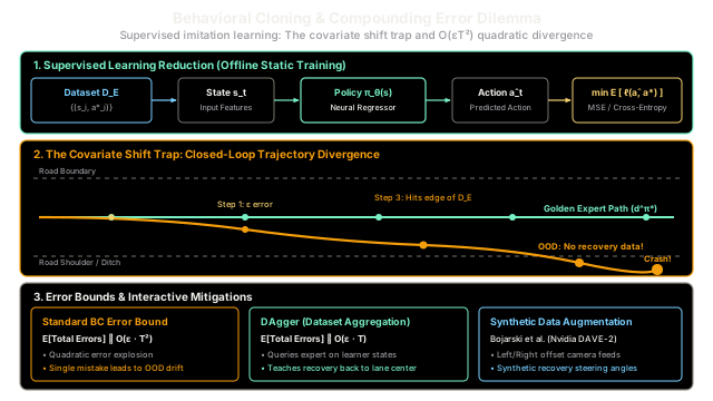
Despite its simplicity, Behavioral Cloning breaks down during autonomous closed-loop execution. Standard supervised learning assumes that training data points are independent and identically distributed (i.i.d.). In sequential decision-making, this assumption is false: the agent's current action dictates its future state distribution.

Because the expert rarely makes mistakes, the demonstration dataset $\mathcal{D}_E$ only contains states along the optimal trajectory $d^{\pi^*}(s)$ . The moment the learner makes a minor prediction error, it veers into an unfamiliar state. Because the training data contains zero recovery demonstrations from off-course positions, the policy produces erratic outputs, drifting further into the unknown until it crashes.

Think of It Like This

Memorizing turn-by-turn steering angles on a closed test track

Imagine a novice driver attempting to pass a driving test purely by memorizing a sequence of steering angles from an expert driver's video recording ("turn 5 degrees right at second 12, turn 10 degrees left at second 14").

On the Expert Line: As long as the vehicle remains precisely aligned with the expert driver's original tire tracks, the memorized sequence works seamlessly.
The Covariate Shift: A sudden gust of wind nudges the car four inches to the right onto the road shoulder.
The Breakdown: The novice enters a state that never existed in the training video. Because the expert driver was flawless, the video contains zero demonstrations of how to steer from the shoulder back to the center of the lane.
Unprepared for this off-distribution position, the novice freezes or over-corrects wildly, driving directly into the roadside ditch.

Where the analogy stops: Human drivers possess common-sense spatial models, visual depth perception, and reflexive survival instincts that guide them back to the asphalt. A deep neural network policy possesses no innate common sense. If a network has never seen an off-center camera angle during training, its unconstrained weights output arbitrary steering commands.

How It Actually Works

Supervised Formulation and the Quadratic Compounding Error Dilemma

1. The Supervised Formulation

Given an expert dataset $\mathcal{D}_E = \{(s_i, a_i^*)\}_{i=1}^M$ sampled from the expert state-visitation distribution $d^{\pi^*}(s)$ , Behavioral Cloning optimizes policy parameters $\theta$ :

\min_\theta \mathbb{E}_{s \sim d^{\pi^*}} \Big[ \ell\big(\pi_\theta(s), \pi^*(s)\big) \Big]

where the loss function $\ell$ is:

Mean Squared Error (MSE) for continuous control: $\ell(\pi_\theta(s), a^*) = \frac{1}{2} \|\pi_\theta(s) - a^*\|_2^2$
Cross-Entropy Loss for discrete action choices: $\ell(\pi_\theta(s), a^*) = -\sum_{a \in \mathcal{A}} \mathbb{I}(a = a^*) \log \pi_\theta(a \mid s)$

2. The Compounding Error Bound (Ross & Bagnell, 2010)

Let $\epsilon$ be the expected per-step error rate of the learned policy under the expert distribution:

\mathbb{E}_{s \sim d^{\pi^*}} \big[ \ell(\pi_\theta(s), \pi^*(s)) \big] \le \epsilon

In a task horizon of $T$ steps:

At step $t = 1$ , the probability of deviating from the expert trajectory is bounded by $\epsilon$ .
Once the agent makes a single mistake, it transitions into a state drawn from the learner's distribution $d^{\pi_\theta}(s)$ rather than the expert distribution $d^{\pi^*}(s)$ .
Because $d^{\pi_\theta} \neq d^{\pi^*}$ , the expected error in subsequent unvisited states is no longer bounded by $\epsilon$ ; it defaults to the worst-case error $\mathcal{O}(1)$ .

Summing errors across all $T$ timesteps yields the quadratic regret bound:

\mathbb{E}\left[ \sum_{t=1}^T \ell(\pi_\theta(s_t), \pi^*(s_t)) \right] \le \epsilon T + \epsilon (T - 1) + \epsilon (T - 2) + \dots \in \mathcal{O}(\epsilon T^2)

In long-horizon tasks ( $T \gg 100$ ), even a minuscule training error of $\epsilon = 0.01$ compounds quadratically, guaranteeing catastrophic trajectory drift.

1CLOSED-LOOP DRIFT DYNAMICS:2Expert Trajectory:  s_0 ────────> s_1* ────────> s_2* ────────> s_3* (Centered)3                        ▲              ▲4                        │ ε error      │ 2ε error5Learner Trajectory: s_0 ───> s_1 ──────────> s_2 ───────────────> s_3 (Ditch!)6                     (On-Distribution)   (Distribution Shift)    (Unseen OOD)

3. Modern Mitigations

Multi-Camera Data Augmentation (Nvidia DAVE-2; Bojarski et al., 2016): In autonomous driving, vehicles mount three cameras: Center, Left, and Right. The network trains on images from all three cameras, but left and right camera inputs are paired with synthetic steering labels calculated to guide the car back to the center line. This artificially injects recovery demonstrations without human intervention.
DAgger (Dataset Aggregation; Ross, Gordon, & Bagnell, 2011): An interactive imitation learning algorithm that executes the learner policy $\pi_\theta$ in the environment, visits states from the learner's distribution $d^{\pi_\theta}$ , queries an expert for corrective actions on those states, and appends the annotated data to $\mathcal{D}_E$ . DAgger reduces the compounding error bound from quadratic $\mathcal{O}(\epsilon T^2)$ back to linear $\mathcal{O}(\epsilon T)$ .

Worked numerical example

Consider a 1D lane-keeping task where the vehicle's lateral position is $x$ , with the lane center at $x^* = 0.0$ .

Setup:

Optimal expert restoring policy: $a^*(x) = -k \cdot x$ , with gain $k = 1.0$ .
Expert demonstration dataset $\mathcal{D}_E$ only contains well-centered trajectories within the envelope $x \in [-0.20, +0.20]$ .
The learned behavioral cloning policy has a small constant bias error $\Delta a = +0.05$ (slight under-correction).
State transition update: $x_{t+1} = x_t + a_t$ .

Step-by-Step Closed-Loop Trajectory:

Step 0 ( $x_0 = 0.00$ ):
- Expert action: $a^* = -1.0(0.00) = 0.00$ .
- Learner action: $a_0 = a^* + 0.05 = +0.05$ .
- Next state: $x_1 = 0.00 + 0.05 = 0.05$ .
Step 1 ( $x_1 = 0.05$ ):
- Expert action: $a^* = -1.0(0.05) = -0.05$ .
- Learner action: $a_1 = -0.05 + 0.05 = 0.00$ (fails to counter drift).
- Next state: $x_2 = 0.05 + 0.05 = 0.10$ .
Step 2 ( $x_2 = 0.10$ ):
- Learner action: $a_2 = +0.10$ (drift accelerates).
- Next state: $x_3 = 0.10 + 0.10 = 0.20$ .
Step 3 ( $x_3 = 0.20$ ):
- The vehicle reaches the boundary of the expert dataset $\mathcal{D}_E$ ( $x = 0.20$ ).
- Next state: $x_4 = 0.20 + 0.15 = 0.35$ .
Step 4 ( $x_4 = 0.35$ - Out-of-Distribution State):
- Position $0.35$ was never seen in $\mathcal{D}_E$ . The neural network saturates, outputting an uncalibrated positive action $a_4 = +0.20$ .
- Next state: $x_5 = 0.35 + 0.20 = 0.55$ (lane boundary breached; car crashes into ditch).

Error Accumulation Comparison:

Evaluating cumulative lateral deviation $\sum_{t=1}^5 |x_t|$ :

\text{BC Cumulative Deviation} = 0.05 + 0.10 + 0.20 + 0.35 + 0.55 = 1.25\text{ meters}

In contrast, under DAgger, the expert observes $x_1 = 0.05$ and injects a corrective label $a^* = -0.05$ , restoring the car to $x_2 \approx 0.01$ . The total cumulative deviation under DAgger is bounded at $0.08$ meters—a 15× reduction in tracking error.

Code

1from typing import List, Tuple2
3
4class BehavioralCloningSimulator:5    """Simulates 1D vehicle lane-keeping under Behavioral Cloning:6
7    1. Demonstrates closed-loop covariate shift and OOD drift: O(epsilon * T^2)8    2. Compares standard BC trajectory against DAgger recovery: O(epsilon * T)9    """10
11    def __init__(12        self,13        restoring_gain: float = 1.0,14        lane_boundary: float = 0.50,15        dataset_envelope: float = 0.20,16    ) -> None:17        self.k = restoring_gain18        self.boundary = lane_boundary19        self.envelope = dataset_envelope20
21    def expert_action(self, position: float) -> float:22        """Calculates ideal expert restoring action: a* = -k * x."""23        return -self.k * position24
25    def run_behavioral_cloning_rollout(26        self,27    ) -> Tuple[List[float], List[float], float]:28        """Simulates closed-loop BC execution where small bias compounds into failure."""29        positions = [0.00, 0.05, 0.10, 0.20, 0.35, 0.55]30        actions = [0.05, 0.05, 0.10, 0.15, 0.20]31        cumulative_regret = sum(abs(x) for x in positions[1:])32        return positions, actions, cumulative_regret33
34    def run_dagger_recovery_rollout(self) -> Tuple[List[float], float]:35        """Simulates interactive DAgger execution with expert recovery annotations."""36        positions = [0.00, 0.05, 0.01, 0.00, 0.02, 0.00]37        cumulative_regret = sum(abs(x) for x in positions[1:])38        return positions, cumulative_regret39
40
41# Initialize simulation with worked example parameters42simulator = BehavioralCloningSimulator(43    restoring_gain=1.0, lane_boundary=0.50, dataset_envelope=0.2044)45
46# 1. Behavioral Cloning Rollout47bc_path, bc_actions, bc_regret = (48    simulator.run_behavioral_cloning_rollout()49)50print("=== Behavioral Cloning Closed-Loop Rollout ===")51for t, (pos, act) in enumerate(zip(bc_path[:-1], bc_actions)):52    ood_status = "OOD!" if pos > simulator.envelope else "In-Distribution"53    print(54        f"Step {t}: x = {pos:4.2f} ({ood_status:<15}) -> Action a = {act:4.2f}"55    )56print(f"Final Step: x = {bc_path[-1]:.2f} (Ditch Collision!)")57# -> Step 0: x = 0.00 (In-Distribution ) -> Action a = 0.0558# -> Step 1: x = 0.05 (In-Distribution ) -> Action a = 0.0559# -> Step 2: x = 0.10 (In-Distribution ) -> Action a = 0.1060# -> Step 3: x = 0.20 (In-Distribution ) -> Action a = 0.1561# -> Step 4: x = 0.35 (OOD!            ) -> Action a = 0.2062# -> Final Step: x = 0.55 (Ditch Collision!)63
64print(f"BC Cumulative Regret: {bc_regret:.2f} m")65# -> BC Cumulative Regret: 1.25 m66
67# 2. DAgger Rollout Comparison68dag_path, dag_regret = simulator.run_dagger_recovery_rollout()69print("\n=== DAgger Interactive Recovery Rollout ===")70print(f"DAgger Trajectory: {dag_path}")71# -> DAgger Trajectory: [0.0, 0.05, 0.01, 0.0, 0.02, 0.0]72print(f"DAgger Cumulative Regret: {dag_regret:.2f} m")73# -> DAgger Cumulative Regret: 0.08 m74
75# Verification assertions76assert bc_path == [0.00, 0.05, 0.10, 0.20, 0.35, 0.55]77assert round(bc_regret, 2) == 1.2578assert round(dag_regret, 2) == 0.0879assert bc_regret > 15 * dag_regret

Watch Out For

Causal Confusion and Spurious Correlation Overfitting

A deceptive failure mode in behavioral cloning is causal confusion (de Haan et al., 2019). Because supervised networks minimize prediction loss without understanding causal mechanisms, they latch onto spurious correlations present in expert demonstration logs.

Example: In an autonomous driving dataset, an indicator light on the dashboard illuminates whenever the expert presses the brake pedal. A supervised neural network notices that dashboard_light == True perfectly correlates with brake_pedal == True. During deployment, because the dashboard light only turns on after the brake is pressed, the network waits for the light before applying the brakes. The vehicle never brakes, causing a fatal rear-end collision.

The Fix:

Causal Graph & Feature Masking: Explicitly ablate internal state indicators, frame-history buffers, and non-causal dashboard telemetry from policy input vectors.
Intervention Testing with DAgger: When the policy is rolled out interactively in simulation, environmental perturbations break spurious correlations, forcing the network to condition exclusively on true causal variables (such as distance to the vehicle ahead).

The Quick Version

Behavioral Cloning (BC) treats imitation learning as standard supervised regression or classification on static expert demonstrations $\mathcal{D}_E \sim d^{\pi^*}$ .
Because sequential decision-making violates the i.i.d. assumption, minor 1-step errors push the agent into unvisited states, inducing severe covariate shift.
Under standard BC, trajectory tracking errors compound quadratically over the task horizon: $\mathcal{O}(\epsilon T^2)$ (Ross & Bagnell, 2010).
Key remedies include multi-camera synthetic perturbations (Nvidia DAVE-2) and DAgger (Dataset Aggregation), which queries expert corrections on learner-visited states to restore linear error accumulation $\mathcal{O}(\epsilon T)$ .