Dataset Aggregation (DAgger)

Why Does This Exist?

Imitation learning allows autonomous agents to master complex behaviors from expert demonstrations without requiring hand-engineered reward functions. The simplest approach—Behavioral Cloning (BC)—treats imitation as standard supervised learning: it collects a dataset of expert state-action pairs $\mathcal{D} = \{(s, a^*)\}$ and trains a regression or classification policy $\hat{\pi}(a \mid s)$ via empirical risk minimization.

However, Behavioral Cloning suffers from a catastrophic theoretical pathology known as covariate shift:

• Supervised learning assumes training data and testing data are drawn independent and identically distributed (i.i.d.) from the same static distribution.
• In sequential decision problems, states are distinctly non-i.i.d.: the action chosen at time $t$ directly dictates the distribution of states encountered at time $t+1$.

When a cloned policy is deployed in the environment, it inevitably makes small approximation mistakes. Suppose the policy has an per-step error probability of $\epsilon$. At the first mistake, the system transitions into an unfamiliar, slightly abnormal state that the flawless expert never visited.

Because the training set contains zero demonstrations showing how to recover from this off-distribution state, the policy makes an even worse decision. Errors compound exponentially over time. Over an execution horizon of $T$ time steps, the expected cumulative error scales quadratically:

In autonomous driving or robotic flight, this quadratic error accumulation manifests as vehicle drift, lane departure, and catastrophic crashes within seconds.

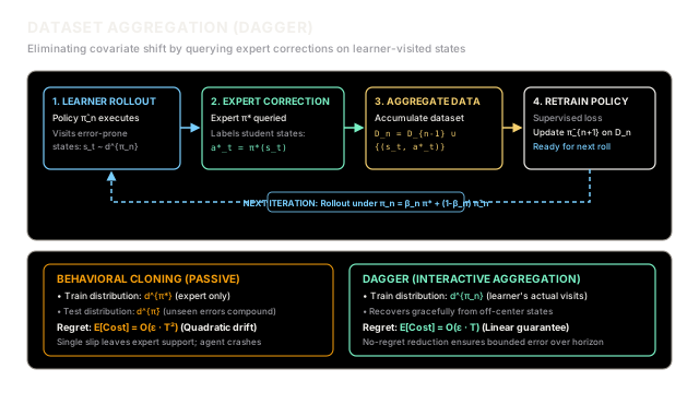
Introduced by Stéphane Ross, Geoffrey Gordon, and J. Andrew Bagnell (2011), Dataset Aggregation (DAgger) solves covariate shift by reframing imitation learning as a reduction to no-regret online learning. Instead of gathering all demonstrations upfront, DAgger allows the imperfect learner to execute rollouts, visit its own error-prone states, and interactively query the expert for corrective labels, bounding total errors linearly to $\mathcal{O}(\epsilon \cdot T)$.

Think of It Like This

How It Actually Works

The Compounding Error Derivation of Behavioral Cloning

To understand why DAgger is necessary, consider an agent with a per-step error probability $\epsilon$:

where $d^{\pi^*}$ is the state distribution induced by running the expert policy.

Let the 0-1 loss at each step be $\ell(s, a, a^*) \in \{0, 1\}$. Under Behavioral Cloning:

• At time step $t=1$, the probability of mistake is $\epsilon$.
• If the agent makes a mistake, it enters a state unvisited by the expert. Under worst-case dynamics, it can incur a cost of $1$ for all remaining $T - t$ time steps.
• Summing the expected cost over horizon $T$: $$J(\hat{\pi}) \le \sum_{t=1}^T \mathbb{P}(\text{first error at step } t) \cdot (T - t + 1) \le \sum_{t=1}^T \epsilon (1 - \epsilon)^{t-1} (T - t + 1)$$ For small $\epsilon$, this sum evaluates to: $$J(\hat{\pi}) \le \epsilon T + \epsilon(T-1) + \epsilon(T-2) + \dots \approx \frac{\epsilon T^2}{2} = \mathcal{O}\left(\epsilon \cdot T^2\right)$$

The quadratic penalty arises because the training distribution $d^{\pi^*}$ differs fundamentally from the deployment distribution $d^{\hat{\pi}}$.

The DAgger Interactive Loop

DAgger resolves this mismatch by training the policy directly on the state distribution that the policy itself induces, $d^{\hat{\pi}}$.

The algorithm proceeds across $N$ outer iterations:

1. Iteration 1 (Initial Demonstration):

   • Gather an initial trajectory dataset using the expert policy $\pi^*$: $$\mathcal{D}_1 = \left\{ \left(s_t, \pi^*(s_t)\right) \right\}_{t=1}^T$$
   • Train an initial supervised policy $\hat{\pi}_1 = \arg\min_{\pi \in \Pi} \frac{1}{|\mathcal{D}_1|} \sum_{(s, a^*) \in \mathcal{D}_1} \ell\left(s, \pi(s), a^*\right)$.

2. Iterations $n = 2, \dots, N$:

   • Define a mixed execution policy: $$\pi_n = \beta_n \pi^* + (1 - \beta_n) \hat{\pi}_n$$ where $\beta_n \in [0, 1]$ is a mixing coefficient. In practice, $\beta_n = p^{n-1}$ (with $p < 1$), decaying to $0$ so the learner rapidly drives fully autonomously.
   • Roll out policy $\pi_n$ in the environment to generate a trajectory of visited states: $$\tau_n = \left( s_1, s_2, \dots, s_T \right) \sim d^{\pi_n}$$
   • Query the Expert: For every state $s_t \in \tau_n$ visited by the learner, query the expert for the optimal corrective action $a_t^* = \pi^*(s_t)$.
   • Dataset Aggregation: Append the newly labeled transitions to the cumulative training pool: $$\mathcal{D}_n = \mathcal{D}_{n-1} \cup \left\{ \left(s_t, \pi^*(s_t)\right) \right\}_{t=1}^T$$
   • Supervised Retraining: Retrain policy $\hat{\pi}_{n+1}$ on the aggregated dataset $\mathcal{D}_n$ using standard supervised loss (e.g., Mean Squared Error or Cross-Entropy).

Theoretical Guarantee via No-Regret Reduction

Because the dataset aggregates states visited across all iterations, the empirical training distribution approaches the average learner distribution $\frac{1}{N} \sum_{n=1}^N d^{\pi_n}$.

By viewing this iterative process through the lens of online convex optimization (Follow the Leader), Ross, Gordon, and Bagnell proved that if the supervised learning algorithm achieves an average training loss $\epsilon_N = \frac{1}{N} \sum_{n=1}^N \epsilon_n$, then as $N \to \infty$ and $\beta_n \to 0$:

This translates to a strictly linear bound on the cumulative expected cost over the horizon $T$:

where $u$ is a task-dependent loss constant. DAgger completely eliminates the quadratic $\mathcal{O}(\epsilon T^2)$ failure mode of Behavioral Cloning.

Worked numerical example

Consider a 1D continuous lane-keeping task.

• State $x \in [-1.0, 1.0]$ is the vehicle's lateral deviation from the lane center ($x = 0$ is optimal).
• Action $a \in [-1.0, 1.0]$ is the steering angle.
• The environment has simple kinematic dynamics: $x_{t+1} = x_t + a_t$.
• The expert controller is an optimal proportional centering policy: $\pi^*(x) = -x$.

1. Behavioral Cloning Phase (Iteration 1)

The expert provides demonstrations strictly near the center line: $7$ sample points uniformly spaced in $x \in [-0.10, 0.10]$ with actions $a^* = -x$. Using a localized function approximator (e.g., Radial Basis Functions with centers across the domain), the policy is fit via regularized least squares on $\mathcal{D}_1$.

Now, an external disturbance pushes the vehicle onto the shoulder at $x_0 = 0.400$. We evaluate the BC policy over $3$ autonomous steps:

• Step 0 ($x_0 = 0.400$):
  • Expert action would be $\pi^*(0.400) = -0.400$.
  • Because $x = 0.400$ is far outside the $[-0.10, 0.10]$ training support, the BC policy under-steers severely, predicting $a_0 = -0.109$.
  • Next state: $x_1 = 0.400 + (-0.109) = 0.291$.
  • Squared error on this shoulder state: $$\text{MSE}_{\text{BC}} = \left( a_0 - a^* \right)^2 = \left( -0.109 - (-0.400) \right)^2 = (0.291)^2 \approx 0.0847$$
• Step 1 ($x_1 = 0.291$):
  • BC predicts $a_1 = -0.150 \implies x_2 = 0.291 - 0.150 = 0.141$.
• Step 2 ($x_2 = 0.141$):
  • BC predicts $a_2 = -0.127 \implies x_3 = 0.141 - 0.127 = 0.014$.

Notice that the vehicle drifts across multiple steps before slowly returning, accumulating large lateral deviations.

2. DAgger Interactive Aggregation (Iteration 2)

In DAgger, the learner visited the sequence of off-center states $\{0.400, 0.291, 0.141\}$. The algorithm queries the expert for optimal actions at these three student-visited states:

• At $x = 0.400 \implies a^* = -0.400$
• At $x = 0.291 \implies a^* = -0.291$
• At $x = 0.141 \implies a^* = -0.141$

These $3$ corrective pairs are appended to $\mathcal{D}_1$, expanding the dataset to $\mathcal{D}_2$ ($10$ transitions). The policy is retrained on $\mathcal{D}_2$.

3. Re-evaluating Retrained Policy

Deploy the updated policy $\hat{\pi}_2$ from the same shoulder perturbation $x_0 = 0.400$:

• Step 0 ($x_0 = 0.400$):
  • The retrained policy now recognizes the shoulder state and outputs $a_0 = -0.396$.
  • Next state: $x_1 = 0.400 + (-0.396) = 0.004$.
  • Squared error: $$\text{MSE}_{\text{DAgger}} = \left( -0.396 - (-0.400) \right)^2 = (0.004)^2 \approx 0.000016$$
• Step 1 ($x_1 = 0.004$):
  • Policy predicts $a_1 = -0.005 \implies x_2 = 0.004 - 0.005 = -0.001$.
• Step 2 ($x_2 = -0.001$):
  • Policy predicts $a_2 = 0.001 \implies x_3 = 0.000$.

By aggregating just $3$ corrective samples from the learner's own rollout, the shoulder MSE plummeted from $0.0847 \to 0.000016$. The vehicle recovers back to center in a single step rather than sluggishly drifting.

Code

The following self-contained Python implementation simulates the DAgger algorithm on a continuous lane-keeping task, comparing initial Behavioral Cloning against interactive dataset aggregation.

1from typing import Callable, List, Tuple2import numpy as np3
4
5class DAggerSimulator:6    """7    Simulation of Dataset Aggregation (DAgger) on a continuous lane-keeping task.8    Demonstrates how querying expert labels on learner-visited states9    mitigates covariate shift.10    """11
12    def __init__(self, expert_fn: Callable[[float], float]) -> None:13        self.expert_fn = expert_fn14        self.dataset: List[Tuple[float, float]] = []15        # Radial basis centers spanning the operating domain16        self.centers = np.array([-0.4, -0.2, -0.1, 0.0, 0.1, 0.2, 0.4])17        self.gamma = 25.018        self.weights = np.zeros(len(self.centers))19
20    def _features(self, x: float) -> np.ndarray:21        """Extracts localized Radial Basis Function features."""22        return np.exp(-self.gamma * (x - self.centers) ** 2)23
24    def train_policy(self) -> None:25        """Fits policy weights using regularized least squares on self.dataset."""26        if not self.dataset:27            return28        X = np.array([self._features(pt[0]) for pt in self.dataset])29        y = np.array([pt[1] for pt in self.dataset])30        reg = 1e-3 * np.eye(X.shape[1])31        self.weights = np.linalg.solve(X.T @ X + reg, X.T @ y)32
33    def predict(self, x: float) -> float:34        """Evaluates learned policy on state x."""35        return float(self._features(x) @ self.weights)36
37    def rollout(38        self, start_x: float, steps: int = 339    ) -> List[Tuple[float, float, float]]:40        """41        Executes autonomous policy in environment: x_{t+1} = x_t + a_t42        Returns list of (state, learner_action, next_state).43        """44        trajectory = []45        x = start_x46        for _ in range(steps):47            a = self.predict(x)48            next_x = x + a49            trajectory.append((x, a, next_x))50            x = next_x51        return trajectory52
53    def run_demonstration(self) -> None:54        np.random.seed(42)55        print("=== 1. INITIAL BEHAVIORAL CLONING (BC) PHASE ===")56        # Expert demonstrates only on lane center states: x in [-0.10, +0.10]57        initial_states = np.linspace(-0.10, 0.10, 7)58        for s in initial_states:59            self.dataset.append((float(s), self.expert_fn(float(s))))60
61        self.train_policy()62        print(f"Initial Dataset D_1 Size: {len(self.dataset)} expert transitions")63
64        # Evaluate BC on off-distribution shoulder perturbation (x = 0.40)65        bc_traj = self.rollout(start_x=0.40, steps=3)66        print("\nBC Rollout from shoulder (x = 0.40):")67        for t, (s, a, next_s) in enumerate(bc_traj):68            print(f"  Step {t}: x = {s:.3f} -> a = {a:.3f} -> next_x = {next_s:.3f}")69
70        loss_shoulder_bc = (bc_traj[0][1] - self.expert_fn(0.40)) ** 271        print(f"MSE on shoulder state x=0.40 under BC: {loss_shoulder_bc:.4f}")72
73        print("\n=== 2. DAGGER INTERACTIVE AGGREGATION PHASE ===")74        # Query expert on every state visited by the learner during its rollout75        print("Querying expert on learner-visited states:")76        for s, learner_a, _ in bc_traj:77            expert_a = self.expert_fn(s)78            self.dataset.append((s, expert_a))79            print(80                f"  State x = {s:.3f} | Learner a = {learner_a:.3f} | "81                f"Expert correction a* = {expert_a:.3f}"82            )83
84        # Retrain policy on aggregated dataset D_285        self.train_policy()86        print(f"\nAggregated Dataset D_2 Size: {len(self.dataset)} transitions")87
88        # Re-evaluate retrained policy from the same shoulder perturbation89        dagger_traj = self.rollout(start_x=0.40, steps=3)90        print("\nDAgger Rollout from shoulder (x = 0.40):")91        for t, (s, a, next_s) in enumerate(dagger_traj):92            print(f"  Step {t}: x = {s:.3f} -> a = {a:.3f} -> next_x = {next_s:.3f}")93
94        loss_shoulder_dagger = (dagger_traj[0][1] - self.expert_fn(0.40)) ** 295        print(f"MSE on shoulder state x=0.40 under DAgger: {loss_shoulder_dagger:.6f}")96
97
98if __name__ == "__main__":99    # Centering expert policy: a* = -x100    expert_controller = lambda x: -x101    sim = DAggerSimulator(expert_fn=expert_controller)102    sim.run_demonstration()

Output:

1=== 1. INITIAL BEHAVIORAL CLONING (BC) PHASE ===2Initial Dataset D_1 Size: 7 expert transitions3
4BC Rollout from shoulder (x = 0.40):5  Step 0: x = 0.400 -> a = -0.109 -> next_x = 0.2916  Step 1: x = 0.291 -> a = -0.150 -> next_x = 0.1417  Step 2: x = 0.141 -> a = -0.127 -> next_x = 0.0138MSE on shoulder state x=0.40 under BC: 0.08479
10=== 2. DAGGER INTERACTIVE AGGREGATION PHASE ===11Querying expert on learner-visited states:12  State x = 0.400 | Learner a = -0.109 | Expert correction a* = -0.40013  State x = 0.291 | Learner a = -0.150 | Expert correction a* = -0.29114  State x = 0.141 | Learner a = -0.127 | Expert correction a* = -0.14115
16Aggregated Dataset D_2 Size: 10 transitions17
18DAgger Rollout from shoulder (x = 0.40):19  Step 0: x = 0.400 -> a = -0.396 -> next_x = 0.00420  Step 1: x = 0.004 -> a = -0.005 -> next_x = -0.00121  Step 2: x = -0.001 -> a = 0.001 -> next_x = -0.00022MSE on shoulder state x=0.40 under DAgger: 0.000017

Watch Out For

The Quick Version

• Eliminates Covariate Shift: Behavioral Cloning suffers from compounding out-of-distribution drift $\mathcal{O}(\epsilon T^2)$ because training and test distributions differ; DAgger aligns them to guarantee linear regret $\mathcal{O}(\epsilon T)$.
• Interactive Correction: The learner executes trajectories in the environment, visits its own error-prone states, and queries the expert for optimal actions on those exact states.
• Dataset Accumulation: New expert-labeled transitions are continually aggregated into a growing dataset $\mathcal{D}_n$, training the policy to actively recover from mistakes.
• Query Burden Mitigation: To avoid overwhelming human demonstrators with thousands of queries, modern extensions like Safe DAgger gate expert requests based on epistemic policy uncertainty.

What to Read Next

• Behavioral Cloning
• Imitation Learning
• Generative Adversarial Imitation Learning (GAIL)