Conditional Value at Risk (CVaR) Optimization

Why Does This Exist?

Standard RL chases the mean. It picks the policy with the highest expected return and calls it done. That works until the mean hides a cliff edge.

Picture two delivery robot policies. Both average +4.3 per shift. One never drops below -2. The other scores +22 on lucky shifts and -20 when it tips down stairs. A mean-only optimizer calls them tied. Your hardware budget does not. You want the policy whose worst fifth of shifts still pays, even if its highlight reel looks plainer.

That is what this page covers. You will see how VaR marks the edge of the bad tail and how CVaR averages everything past that edge, with a 10-episode worked example you can check by hand. It then sketches how a policy gradient lifts that tail.

Two neighbours do the adjacent jobs. Quantile Regression DQN teaches how to estimate the return distribution that VaR and CVaR read from. Safe RL teaches how to add hard constraints during training and deployment. This page teaches the tail objective itself, the workhorse of risk-sensitive RL. For the fixed-grid distribution that started this family, see Categorical DQN.

You only need one prerequisite idea. Each episode produces a total discounted return $R$. Run the same policy ten times and you get ten different $R$ values because starts, noise, and slips differ. VaR and CVaR are just two ways of summarizing the low end of those numbers.

Think of It Like This

How It Actually Works

Let $R$ be the random episodic return under policy $\pi_\theta$, where $\theta$ holds the policy weights. Let $F(r) = P(R \le r)$ be its cumulative distribution, so $F(r)$ is the chance a return lands at or below $r$. Let $\alpha$ in $(0, 1)$ be the tail fraction you care about, here $0.2$ for the worst fifth.

VaR marks the edge, CVaR averages past it

VaR (Value at Risk) is the quantile at $\alpha$:

$VaR_\alpha = \inf \{ r : F(r) \ge \alpha \}$

In plain words, $VaR_\alpha$ is the cutoff where the worst $\alpha$ fraction begins. With $\alpha = 0.2$, about 20 percent of episodes score at or below VaR.

CVaR (Conditional Value at Risk) is the mean inside that tail:

$CVaR_\alpha = E[R \mid R \le VaR_\alpha] = \frac{1}{\alpha} \int_0^\alpha VaR_u \, du$

So VaR is one number on the edge, while CVaR averages the whole bad slice. CVaR is always at or below VaR for returns, which is why traders say VaR tells you where the cliff starts and CVaR tells you how deep the drop is.

One convention trap to fix now: finance often defines CVaR on losses with $\alpha = 0.95$ and averages the worst 5 percent above a high quantile. Here we define it on returns and average the worst $\alpha$ below a low quantile. Same idea, mirrored axis. Always check which side the author averages.

Optimization uses a handy variational form from Rockafellar and Uryasev. For returns:

$CVaR_\alpha = \max_\eta \left\{ \eta - \frac{1}{\alpha} E[(\eta - R)_+] \right\}$

Here $\eta$ is a free threshold guess and $(\eta - R)_+ = \max(0, \eta - R)$ is the shortfall below it. The best $\eta$ lands exactly on $VaR_\alpha$. That form matters because it turns a conditional average into an expectation you can sample.

Worked example with 10 sampled returns

Say one policy produces these 10 episode returns, in the order they happened:

$[12, 5, -8, 22, 3, -20, 9, 15, -2, 7]$

Sort them lowest first:

$[-20, -8, -2, 3, 5, 7, 9, 12, 15, 22]$

The plain mean is:

$(43) / 10 = 4.3$

since the values sum to $43$. A mean-only reader sees +4.3 and moves on.

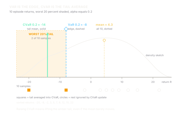
Now take $\alpha = 0.2$. The tail holds $\alpha \times 10 = 2$ episodes. Using the order-statistic rule, VaR is the second smallest value:

$VaR_{0.2} = -8$

CVaR averages the two tail values:

$CVaR_{0.2} = \frac{-20 + (-8)}{2} = \frac{-28}{2} = -14$

So the policy averages +4.3 overall but -14 across its worst fifth. That gap is the whole argument for CVaR: the mean says fine, the tail says fix the stairs fall first. The diagram at the top draws these same numbers, with VaR as the dashed edge and CVaR as the solid tail mean left of it.

How a policy gradient lifts the tail

A CVaR policy gradient keeps the tail and mostly ignores the rest. In each update:

1. Roll out $N$ episodes and collect returns $R_1$ to $R_N$.
2. Estimate $VaR_\alpha$ as the empirical $\alpha$-quantile, exactly as above.
3. Keep only episodes with $R_i \le VaR_\alpha$ and push $\theta$ in the direction that makes those episodes both likelier and higher scoring, weighted by their shortfall $(R_i - VaR_\alpha)$ times the score gradient $\nabla_\theta \log P_\theta$.

You will often see the update written with an indicator $\mathbb{I}(R_i \le VaR_\alpha)$ that zeroes out non-tail episodes, which is why only the bad slice teaches. The threshold $\eta$ from the variational form acts as a built-in baseline, so episodes exactly at VaR contribute nothing.

This costs data. With $\alpha = 0.2$ you throw away four of every five episodes per update, so gradients wobble and small test batches mislead. In practice teams pair the objective with a distributional critic such as Quantile Regression DQN, which reads quantiles straight off learned locations instead of re-sorting thousands of rollouts, and they often warm-start on the mean before tightening $\alpha$. Pick CVaR when rare failures dominate your true cost, such as hardware damage or large trading drawdowns. Stick with the mean when failures are cheap and you need every sample to count.

Code

The snippet below computes the same VaR and CVaR from the worked example. It is short on purpose: sort, cut the tail, average it.

1from typing import List, Tuple2
3
4def var_cvar(returns: List[float], alpha: float = 0.2) -> Tuple[float, float, float]:5    """Return (mean, VaR_alpha, CVaR_alpha) for lower-tail returns."""6    ordered = sorted(returns)7    n = len(ordered)8    mean = sum(ordered) / n9    # Order-statistic quantile: first index whose CDF reaches alpha.10    k = max(1, int(-(-alpha * n // 1)))  # ceil(alpha * n)11    var = ordered[k - 1]12    tail = ordered[:k]13    cvar = sum(tail) / len(tail)14    return mean, var, cvar15
16
17episode_returns = [12, 5, -8, 22, 3, -20, 9, 15, -2, 7]18mean, var, cvar = var_cvar(episode_returns, alpha=0.2)19print(f"sorted: {sorted(episode_returns)}")20print(f"mean: {mean:.1f}")21print(f"VaR_0.2: {var}")22print(f"CVaR_0.2: {cvar:.1f}")23# -> sorted: [-20, -8, -2, 3, 5, 7, 9, 12, 15, 22]24# -> mean: 4.325# -> VaR_0.2: -826# -> CVaR_0.2: -14.0

Watch Out For

The Quick Version

• CVaR optimization maximizes the average return of the worst alpha fraction of episodes instead of the overall mean.
• VaR at level alpha is the cutoff where that worst slice starts, while CVaR is the average inside the slice.
• With returns [12, 5, -8, 22, 3, -20, 9, 15, -2, 7], the mean is 4.3, VaR at 0.2 is minus 8, and CVaR at 0.2 is minus 14.
• A CVaR policy gradient keeps only tail episodes and weights each by its shortfall below VaR.
• Small alpha values give stronger protection but need larger batches because most episodes are discarded each update.

What to Read Next

• Quantile Regression DQN (QR-DQN)
• Safe Reinforcement Learning
• Categorical DQN (C51)