Quantile Regression DQN (QR-DQN)

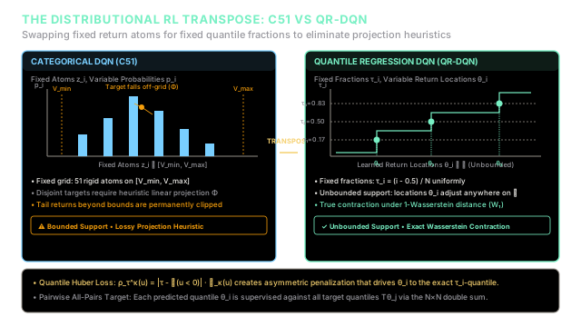
QR-DQN transposes distributional RL by learning variable return locations for fixed quantile fractions, eliminating bounded grids and projection heuristics.

Quantile Regression DQN transposes C51 by fixing uniform quantile fractions along the vertical axis and learning continuous return locations along the horizontal axis.

Why Does This Exist?

In 2017, Categorical DQN (C51, Bellemare et al.) demonstrated that modeling the entire probability distribution of returns $Z(s, a)$ rather than just its expected scalar value $Q(s, a) = \mathbb{E}[Z(s, a)]$ vastly improves representation learning. However, C51 suffered from fundamental architectural limitations:

Rigid Bounded Support: C51 represents returns over a fixed grid of $N=51$ uniformly spaced atoms $\{z_1, \dots, z_{51}\}$ constrained to an arbitrarily chosen interval $[V_{\min}, V_{\max}]$ . If the practitioner chooses poor bounds, or if returns naturally exceed $V_{\max}$ , values outside the interval are permanently clipped, discarding tail risks and catastrophic losses.
Heuristic Projection Step ( $\Phi$ ): When Bellman updates compute target distributions $R + \gamma z_j$ , the discounted atoms almost never land precisely on the predefined grid atoms. C51 must project probability mass onto the two nearest adjacent atoms using linear interpolation. This heuristic projection introduces interpolation noise and breaks the contraction mapping properties of dynamic programming.
Theoretical Disconnect: The distributional Bellman operator $\mathcal{T}^\pi$ is a $\gamma$ -contraction in the $p$ -Wasserstein metric, but the projection operator $\Phi$ used in C51 is not a contraction in Wasserstein distance or Kullback-Leibler divergence.

In 2018, Will Dabney, Mark Rowland, Marc G. Bellemare, and Rémi Munos introduced Quantile Regression DQN (QR-DQN). Their insight was to execute the mathematical transpose of C51:

Instead of fixing the return locations $\{z_i\}$ and learning variable probabilities $\{p_i\}$ , QR-DQN fixes the probabilities to $N$ uniform quantile fractions $\{\tau_1, \dots, \tau_N\}$ and learns variable return locations $\{\theta_1(s, a), \dots, \theta_N(s, a)\} \subset \mathbb{R}$ .

By parameterizing the distribution along the horizontal return axis rather than the vertical probability axis, QR-DQN eliminates $[V_{\min}, V_{\max}]$ bounds, discards heuristic projection entirely, and guarantees theoretical contraction under the $1$ -Wasserstein distance ( $W_1$ ).

Think of It Like This

Slicing the Bread Loaf

Imagine you are tasked with measuring the uneven, heavy-tailed mass distribution of an artisanal loaf of bread:

The C51 Approach (Fixed Baskets): You bolt 51 rigid bread baskets to your countertop at fixed 1-centimeter marks from $0\text{ cm}$ to $50\text{ cm}$ . You slice the bread, but whenever a slice falls at $14.3\text{ cm}$ , it does not fit into any basket. You are forced to crumble the slice and toss $70\%$ into the $14\text{ cm}$ basket and $30\%$ into the $15\text{ cm}$ basket (heuristic projection $\Phi$ ). Worse, if the loaf is longer than $50\text{ cm}$ , any overhang hanging off the edge is sliced off and discarded into the trash (support clipping at $V_{\max}$ ).
The QR-DQN Approach (Equal-Mass Slices): Instead of fixed baskets, you decide to cut the loaf into $N$ slices of strictly equal weight (e.g., $10$ slices, each containing exactly $10\%$ of the bread's total mass). You do not care where the cut marks land—you simply measure the knife positions $\theta_1, \theta_2, \dots, \theta_N$ along the cutting board.

Where the loaf is dense, the cut marks cluster tightly together; where the loaf is airy and sparse, the cut marks spread far apart. The knife can move anywhere along the table without boundaries, slices are never crumbled or projected, and no bread is ever thrown away.

Where the analogy stops: Bread mass is strictly positive and finite. In reinforcement learning, returns can be negative, multi-modal, and unbounded across $(-\infty, +\infty)$ . QR-DQN accommodates arbitrary continuous returns without modifying its quantile target fractions.

How It Actually Works

The Distributional Transpose and Quantile Huber Loss

Let $Z(s, a)$ be the random return variable whose cumulative distribution function (CDF) is $F_Z(z) = \mathbb{P}(Z \le z)$ . The quantile function (or inverse CDF) is defined as:

$F_Z^{-1}(\tau) = \inf \left\{ z \in \mathbb{R} : F_Z(z) \ge \tau \right\}, \quad \text{for } \tau \in (0, 1)$

While C51 approximates the CDF $F_Z(z)$ on a fixed grid of return locations $z$ , QR-DQN approximates the inverse CDF $F_Z^{-1}(\tau)$ by learning $N$ adjustable locations $\theta_1(s, a) \le \dots \le \theta_N(s, a)$ corresponding to fixed uniform quantile target midpoints:

$\hat{\tau}_i = \frac{2i - 1}{2N} = \frac{i - 0.5}{N}, \quad \text{for } i \in \{1, \dots, N\}$

The expected action-value is simply the arithmetic mean of all $N$ learned quantile locations:

$Q(s, a) = \frac{1}{N} \sum_{i=1}^N \theta_i(s, a)$

Quantile Regression and the Huber Smoothing

In statistics, the $\tau$ -th quantile of a distribution minimizes the asymmetric pinball loss (quantile regression loss):

$\rho_\tau(u) = u \left( \tau - \mathbb{I}(u < 0) \right) = \left| \tau - \mathbb{I}(u < 0) \right| |u|$

where $u = \text{target} - \text{prediction}$ , and $\mathbb{I}(\cdot)$ is the indicator function. When $u > 0$ (underestimation), the error is scaled by $\tau$ ; when $u < 0$ (overestimation), the error is scaled by $1 - \tau$ .

However, the standard pinball loss has a non-smooth derivative at $u = 0$ , which causes gradient oscillations when optimizing deep neural networks. Dabney et al. replaced the absolute error $|u|$ with the Huber loss with threshold $\kappa$ :

$\mathcal{L}_\kappa(u) = \begin{cases} \frac{1}{2} u^2 & \text{if } |u| \le \kappa \\ \kappa \left( |u| - \frac{1}{2} \kappa \right) & \text{if } |u| > \kappa \end{cases}$

The resulting Quantile Huber Loss is defined as:

$\rho_\tau^\kappa(u) = \left| \tau - \mathbb{I}(u < 0) \right| \mathcal{L}_\kappa(u)$

For small errors ( $|u| \le \kappa$ ), the loss is quadratic and smooth; for large errors ( $|u| > \kappa$ ), it transitions to linear growth, providing robust gradients.

Pairwise Bellman Target Evaluation

Given a transition $(S_t, A_t, R_{t+1}, S_{t+1})$ :

Action Selection: Select the greedy action using the online network's expected value: $a^* = \arg\max_{a'} Q(S_{t+1}, a') = \arg\max_{a'} \frac{1}{N} \sum_{j=1}^N \theta_j(S_{t+1}, a'; \theta)$
Bellman Target Quantiles: Compute the target locations using the target network $\theta^-$ : $\mathcal{T} \theta_j = R_{t+1} + \gamma \theta_j(S_{t+1}, a^*; \theta^-), \quad \forall j \in \{1, \dots, N\}$
All-Pairs Quantile Huber Loss: Because each target quantile $\mathcal{T} \theta_j$ represents a sample from the target distribution, every predicted quantile $\theta_i(S_t, A_t)$ is evaluated against all $N$ target quantiles: $\mathcal{L}_{\text{QR}}(\theta) = \frac{1}{N} \sum_{i=1}^N \sum_{j=1}^N \rho_{\hat{\tau}_i}^\kappa \left( \mathcal{T} \theta_j - \theta_i(S_t, A_t; \theta) \right)$

The 1-Wasserstein Contraction Guarantee

The $1$ -Wasserstein distance $W_1(F, G)$ between two distributions with inverse CDFs $F^{-1}$ and $G^{-1}$ is:

$W_1(F, G) = \int_0^1 \left| F^{-1}(\tau) - G^{-1}(\tau) \right| d\tau$

The distributional Bellman operator $\mathcal{T}^\pi$ is a $\gamma$ -contraction in $W_1$ :

$W_1(\mathcal{T}^\pi Z_1, \mathcal{T}^\pi Z_2) \le \gamma W_1(Z_1, Z_2)$

Because quantile regression directly projects distributions under the $W_1$ metric without discretization heuristics, QR-DQN preserves contraction mapping guarantees that categorical methods lose.

Worked numerical example

Consider a 3-quantile toy model ( $N = 3$ ) with Huber threshold $\kappa = 1.0$ :

Quantile Fractions: $\hat{\tau}_1 = \frac{1 - 0.5}{3} = \frac{1}{6} \approx 0.1667$ $\hat{\tau}_2 = \frac{2 - 0.5}{3} = \frac{3}{6} = 0.5000$ $\hat{\tau}_3 = \frac{3 - 0.5}{3} = \frac{5}{6} \approx 0.8333$
Current Predicted Quantiles: $\theta(S_t, A_t) = [1.0, 3.0, 5.0]$
Target Network Quantiles at $S_{t+1}$ : $\theta(S_{t+1}, a^*) = [2.0, 4.0, 6.0]$
Transition Dynamics: $R_{t+1} = 1.0$ , discount factor $\gamma = 0.9$ .
Target Quantiles: $\mathcal{T} \theta = 1.0 + 0.9 \times [2.0, 4.0, 6.0] = [2.8, 4.6, 6.4]$

Now compute the pairwise quantile Huber loss for entries in the $3 \times 3$ grid where $u_{ij} = \mathcal{T}\theta_j - \theta_i$ :

Evaluation for First Target $\mathcal{T}\theta_1 = 2.8$ :

Pair $(i=1, j=1)$ : $\theta_1 = 1.0, \mathcal{T}\theta_1 = 2.8, \hat{\tau}_1 = \frac{1}{6}$ $θ_{1} = 1.0, T θ_{1} = 2.8, \overset{τ}{^}_{1} = \frac{1}{6}$
- Error: $u = 2.8 - 1.0 = +1.8$
- Since $|u| = 1.8 > \kappa = 1.0$ : $\mathcal{L}_1(1.8) = 1.0 \times (1.8 - 0.5 \times 1.0) = 1.3000$
- Indicator: $u \ge 0 \implies \mathbb{I}(u < 0) = 0$ . Weight: $|\frac{1}{6} - 0| = \frac{1}{6} \approx 0.1667$
- Loss: $\frac{1}{6} \times 1.3000 = 0.2167$
Pair $(i=2, j=1)$ : $\theta_2 = 3.0, \mathcal{T}\theta_1 = 2.8, \hat{\tau}_2 = 0.5$ $θ_{2} = 3.0, T θ_{1} = 2.8, \overset{τ}{^}_{2} = 0.5$
- Error: $u = 2.8 - 3.0 = -0.2$
- Since $|u| = 0.2 \le \kappa = 1.0$ : $\mathcal{L}_1(-0.2) = 0.5 \times (-0.2)^2 = 0.0200$
- Indicator: $u < 0 \implies \mathbb{I}(u < 0) = 1$ . Weight: $|0.5 - 1| = 0.5000$
- Loss: $0.5 \times 0.0200 = 0.0100$
Pair $(i=3, j=1)$ : $\theta_3 = 5.0, \mathcal{T}\theta_1 = 2.8, \hat{\tau}_3 = \frac{5}{6}$ $θ_{3} = 5.0, T θ_{1} = 2.8, \overset{τ}{^}_{3} = \frac{5}{6}$
- Error: $u = 2.8 - 5.0 = -2.2$
- Since $|u| = 2.2 > \kappa = 1.0$ : $\mathcal{L}_1(-2.2) = 1.0 \times (2.2 - 0.5) = 1.7000$
- Indicator: $u < 0 \implies \mathbb{I}(u < 0) = 1$ . Weight: $|\frac{5}{6} - 1| = \frac{1}{6} \approx 0.1667$
- Loss: $\frac{1}{6} \times 1.7000 = 0.2833$

Full $3 \times 3$ Pairwise Loss Matrix:

0.2167 & 0.5167 & 0.8167 \\ 0.0100 & 0.5500 & 1.4500 \\ 0.2833 & 0.0133 & 0.7500 \end{bmatrix}$$ - **Total Pairwise Loss Sum**: $$\sum_{i=1}^3 \sum_{j=1}^3 L_{ij} = 0.2167 + 0.5167 + 0.8167 + 0.0100 + 0.5500 + 1.4500 + 0.2833 + 0.0133 + 0.7500 = 4.6067$$ - **Mean Loss across all 9 pairs**: $$\bar{\mathcal{L}} = \frac{4.6067}{9} = 0.5119$$ ## Code The following self-contained Python script implements the QR-DQN Quantile Huber loss, evaluates target distributions over $N \times N$ pairwise combinations, and verifies the numerical example with assertions. ```python import numpy as np from typing import Tuple class QRDQNModule: """Computes Quantile Huber Loss and Bellman target updates for QR-DQN.""" def __init__(self, n_quantiles: int = 3, kappa: float = 1.0, gamma: float = 0.9) -> None: self.n = n_quantiles self.kappa = kappa self.gamma = gamma # Midpoint quantile fractions tau_i = (i - 0.5) / N self.tau_hat = np.array([(i - 0.5) / self.n for i in range(1, self.n + 1)]) def quantile_huber_loss( self, target_quantiles: np.ndarray, pred_quantiles: np.ndarray ) -> Tuple[np.ndarray, float]: """Compute pairwise N x N quantile Huber loss matrix and mean loss.""" # diff[i, j] = target[j] - pred[i] diff = target_quantiles[None, :] - pred_quantiles[:, None] abs_diff = np.abs(diff) # Element-wise Huber loss huber = np.where( abs_diff <= self.kappa, 0.5 * (diff ** 2), self.kappa * (abs_diff - 0.5 * self.kappa) ) # Asymmetric quantile weights: |tau_i - I(diff < 0)| indicator = (diff < 0.0).astype(float) tau_weights = np.abs(self.tau_hat[:, None] - indicator) pairwise_loss = tau_weights * huber mean_loss = float(np.mean(pairwise_loss)) return pairwise_loss, mean_loss def run_qrdqn_verification() -> None: qr = QRDQNModule(n_quantiles=3, kappa=1.0, gamma=0.9) # 1. Worked Numerical Example setup theta_current = np.array([1.0, 3.0, 5.0]) reward = 1.0 theta_next = np.array([2.0, 4.0, 6.0]) # Compute Bellman targets: T theta = R + gamma * theta_next t_theta = reward + qr.gamma * theta_next matrix, mean_loss = qr.quantile_huber_loss(t_theta, theta_current) print("--- QR-DQN Loss Evaluation ---") print("Quantile fractions tau_hat: ", np.round(qr.tau_hat, 4)) print("Current predictions theta: ", theta_current) print("Target quantiles T_theta: ", t_theta) print("\nPairwise 3x3 Loss Matrix:") print(np.round(matrix, 4)) print(f"\nMean Pairwise Loss: {mean_loss:.4f}") # Expected values from hand calculation expected_matrix = np.array([ [0.2167, 0.5167, 0.8167], [0.0100, 0.5500, 1.4500], [0.2833, 0.0133, 0.7500] ]) # Automated assertions assert np.allclose(t_theta, [2.8, 4.6, 6.4]), "Target quantiles mismatch" assert np.allclose(matrix, expected_matrix, atol=1e-3), "Loss matrix mismatch" assert np.isclose(mean_loss, 0.5119, atol=1e-3), "Mean loss mismatch" if __name__ == "__main__": run_qrdqn_verification() ``` ```text # -> expected output: --- QR-DQN Loss Evaluation --- Quantile fractions tau_hat: [0.1667 0.5 0.8333] Current predictions theta: [1. 3. 5.] Target quantiles T_theta: [2.8 4.6 6.4] Pairwise 3x3 Loss Matrix: [[0.2167 0.5167 0.8167] [0.01 0.55 1.45 ] [0.2833 0.0133 0.75 ]] Mean Pairwise Loss: 0.5119 ``` ## Watch Out For <PitfallCard title="The Unsorted Quantiles and Huber Threshold Trap"> A critical subtlety when implementing QR-DQN is the **quantile crossing problem**: Because neural networks output $N$ unconstrained continuous numbers $\theta_1(s, a), \dots, \theta_N(s, a)$, nothing in the network architecture mathematically forces the output heads to remain monotonic ($\theta_1 \le \theta_2 \le \dots \le \theta_N$). While the asymmetric quantile Huber loss will statistically encourage proper ordering over training, individual forward passes early in learning or on out-of-distribution states can yield out-of-order predictions ($\theta_1 > \theta_2$). If your agent uses learned distributions for **risk-sensitive policy execution** (such as Conditional Value-at-Risk, CVaR, or worst-decile avoidance), unsorted quantiles will corrupt decision-making. - **The Fix**: Whenever evaluating risk metrics or plotting empirical CDFs, explicitly sort the output vector: ```python sorted_quantiles = np.sort(theta_output, axis=-1) ``` Additionally, practitioners often misconfigure the Huber threshold $\kappa$: - Setting $\kappa \to 0$ reverts to the non-smooth $L_1$ pinball loss, causing gradient jitter around the target. - Setting $\kappa$ excessively large ($\kappa \to \infty$) turns the loss into symmetric mean squared error, destroying the asymmetric penalization that forces $\theta_i$ to its respective quantile. - Keep $\kappa = 1.0$ (or scale $\kappa$ proportionally with reward magnitudes) as recommended by Dabney et al. </PitfallCard> ## The Quick Version - **The Distributional Transpose**: QR-DQN transposes C51 by fixing probabilities to uniform quantile fractions $\tau_i = \frac{i - 0.5}{N}$ and learning continuous return locations $\theta_i(s, a) \in \mathbb{R}$. - **Zero Heuristic Projection**: Eliminates rigid $[V_{\min}, V_{\max}]$ bounds and the lossy projection operator $\Phi$, preventing tail clipping and interpolation noise. - **Quantile Huber Loss**: Combines asymmetric pinball weighting with smooth quadratic Huber loss around zero to provide stable, non-oscillating neural network gradients. - **1-Wasserstein Contraction**: Directly minimizes the $W_1$ distance, preserving dynamic programming contraction guarantees that categorical methods break.