Double DQN (DDQN)

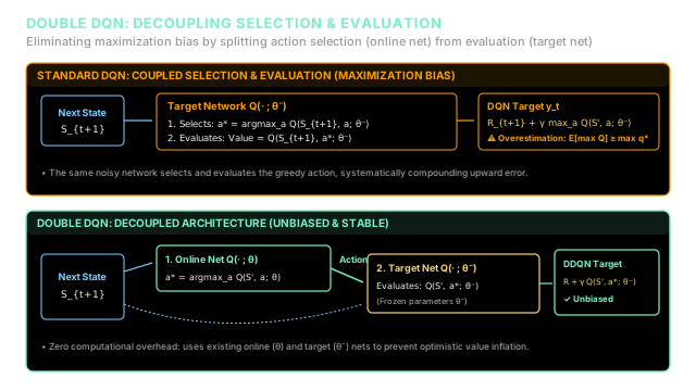
Double DQN eliminates maximization bias by using the online network to pick the best action and the target network to evaluate its value, preventing inflated return estimates.

Double DQN decouples greedy action selection using the online network from value evaluation using the target network, eliminating overestimation bias.

Why Does This Exist?

In value-based reinforcement learning, standard Q-learning suffers from maximization bias. Whenever value estimates are noisy, taking the maximum over estimated action-values systematically overestimates the true maximum value. Mathematically, by Jensen's inequality:

$\mathbb{E} \left[ \max_a Q(S_{t+1}, a) \right] \ge \max_a \mathbb{E} \left[ Q(S_{t+1}, a) \right]$

In deep reinforcement learning, this estimation noise is unavoidable. Stochastic gradient descent, mini-batch sampling, and neural network function approximation errors all introduce zero-mean fluctuations $\epsilon(s, a)$ around true action values:

$Q(s, a; \theta) = q_*(s, a) + \epsilon(s, a)$

In standard Deep Q-Networks (DQN, Mnih et al., 2015), the temporal difference target uses the target network parameters $\theta^-$ for both selecting the greedy action and evaluating its return:

$y^{\text{DQN}}_t = R_{t+1} + \gamma \max_a Q(S_{t+1}, a; \theta^-_t) = R_{t+1} + \gamma Q \left( S_{t+1}, \arg\max_a Q(S_{t+1}, a; \theta^-_t); \theta^-_t \right)$

Because the $\arg\max$ operator inherently selects whichever action happens to have the most positive noise fluctuation $\epsilon(S_{t+1}, a)$ , evaluating that same action with the same network parameters $\theta^-_t$ locks in an upward bias. Across thousands of gradient steps, these inflated targets propagate backward through Bellman updates. In classic Atari benchmarks (such as Asterix, Breakout, and Wizard of Wor), standard DQN frequently inflated Q-values by hundreds of percent above true expected returns, leading to unstable learning dynamics and suboptimal policies.

In 2015, Hado van Hasselt, Arthur Guez, and David Silver introduced Double DQN (DDQN). Their insight was that standard DQN already maintains two distinct sets of weights: the fast-updating online network $\theta$ and the slowly updated target network $\theta^-$ . By simply using the online network to select the action and the target network to evaluate its return, Double DQN completely decouples selection from evaluation. This eliminates systematic overestimation with zero extra neural networks and zero additional memory overhead.

Think of It Like This

The Catalog Curator and the Independent Appraiser

Imagine an art gallery curator trying to purchase high-value antiques from an auction catalog. Every item in the catalog has an uncertain market value subject to noisy estimation.

In standard DQN, the curator acts as both the buyer and the appraiser. The curator flips through the catalog, identifies the item that looks like the biggest bargain based on their own gut feeling, and immediately writes down that same optimistic estimate as the guaranteed resale price in the gallery's ledger. Because the curator selects the item specifically because their estimate was unusually high, their ledger consistently inflates the gallery's net worth. Over time, the gallery goes bankrupt purchasing overvalued inventory.

In Double DQN, the gallery separates the two responsibilities between two individuals:

The Curator (Online Network $\theta$ ): Selects which piece to bid on based on current auction trends ( $a^* = \arg\max_a Q(S', a; \theta)$ ).
The Independent Appraiser (Target Network $\theta^-$ ): Does not choose the item. Instead, they inspect the curator's chosen item and calculate a conservative, independent appraisal ( $Q(S', a^*; \theta^-)$ ).

If the curator was tricked by a random upward valuation error on an inferior painting, the independent appraiser—who has an entirely separate assessment history—will evaluate it without that specific positive error. The gallery's books reflect realistic market values, preventing runaway financial speculation.

Where the analogy stops: The curator and the appraiser are not completely separate entities in deep RL; the appraiser's weights $\theta^-$ are periodically cloned from the curator's weights $\theta$ every few thousand steps. However, because $\theta^-$ is frozen between updates, its instantaneous estimation errors are uncorrelated with the online network's current per-step noise.

How It Actually Works

Maximization Bias and Decoupled Bellman Targets

To understand how Double DQN removes overestimation, compare the Bellman target formulations directly.

Standard DQN Target Formulation

Standard DQN evaluates future returns using a single set of target network weights $\theta^-$ :

$y^{\text{DQN}}_t = R_{t+1} + \gamma Q \left( S_{t+1}, \arg\max_a Q(S_{t+1}, a; \theta^-_t); \theta^-_t \right)$

Here, both the action selection operator $\arg\max_a$ and the value projection $Q(\cdot)$ depend on $\theta^-_t$ .

Double DQN Target Formulation

Double DQN decouples the decision into two distinct stages:

Greedy Action Selection (Online Network $\theta_t$ ): The online network identifies the optimal action for the subsequent state: $a^*(S_{t+1}) = \arg\max_a Q(S_{t+1}, a; \theta_t)$
Action Valuation (Target Network $\theta^-_t$ ): The frozen target network evaluates the expected value of that chosen action: $y^{\text{DDQN}}_t = R_{t+1} + \gamma Q \left( S_{t+1}, a^*(S_{t+1}); \theta^-_t \right)$

Combining these two stages into a single expression:

$y^{\text{DDQN}}_t = R_{t+1} + \gamma Q \left( S_{t+1}, \arg\max_a Q(S_{t+1}, a; \theta_t); \theta^-_t \right)$

The online network parameters $\theta$ are updated via gradient descent on the mean squared temporal difference loss across transitions sampled from replay buffer $\mathcal{D}$ :

$\mathcal{L}(\theta) = \mathbb{E}_{(S_t, A_t, R_{t+1}, S_{t+1}) \sim \mathcal{D}} \left[ \left( y^{\text{DDQN}}_t - Q(S_t, A_t; \theta) \right)^2 \right]$

The target network weights $\theta^-$ remain frozen and are synchronized periodically every $C$ steps ( $\theta^- \leftarrow \theta$ ), or updated via Polyak averaging:

$\theta^- \leftarrow \tau \theta + (1 - \tau) \theta^-, \quad \text{with } \tau \ll 1$

Algorithmic Comparison

Component	Standard DQN	Tabular Double Q-Learning	Double DQN (DDQN)
Action Selection Net	Target Network $\theta^-$	Randomized Choice ( $\theta^A$ or $\theta^B$ )	Online Network $\theta$
Action Evaluation Net	Target Network $\theta^-$	Opposite Network ( $\theta^B$ or $\theta^A$ )	Target Network $\theta^-$
Additional Weights	None	Requires 2 full tables ( $2 \times \vert\mathcal{S}\vert \times \vert\mathcal{A}\vert$ )	Zero additional networks (reuses $\theta^-$ )
Maximization Bias	Severe upward inflation	Unbiased ( $\mathbb{E}[Q] \approx q_*$ )	Unbiased ( $\mathbb{E}[Q] \approx q_*$ )

Worked numerical example

To see the mathematical difference, consider a concrete numerical transition where ground-truth action values are identical, meaning any difference between actions is pure estimation noise:

Next State: $S_{t+1}$ with two candidate actions: $\mathcal{A} = \{a_1, a_2\}$ .
True Values: $q_*(S_{t+1}, a_1) = 0.0$ and $q_*(S_{t+1}, a_2) = 0.0$ .
Environment Transition: Immediate reward $R_{t+1} = 1.0$ , discount factor $\gamma = 0.9$ .
True Bellman Target: $y^* = R_{t+1} + \gamma \max_a q_*(S_{t+1}, a) = 1.0 + 0.9(0.0) = 1.0000$

Due to stochastic training gradients, the networks produce slightly noisy estimates:

Online Network $\theta$ : $Q(S_{t+1}, a_1; \theta) = +0.50, \quad Q(S_{t+1}, a_2; \theta) = -0.30$
Target Network $\theta^-$ : $Q(S_{t+1}, a_1; \theta^-) = -0.20, \quad Q(S_{t+1}, a_2; \theta^-) = +0.60$

Step 1: Standard DQN Target Calculation

Standard DQN queries the target network $\theta^-$ to select and evaluate:

Selection: $a_{\text{DQN}}^* = \arg\max_a Q(S_{t+1}, a; \theta^-) = \arg\max \{ -0.20, +0.60 \} = a_2$
Evaluation: $Q(S_{t+1}, a_2; \theta^-) = +0.60$
Target: $y^{\text{DQN}} = R_{t+1} + \gamma Q(S_{t+1}, a_2; \theta^-) = 1.0 + 0.9(+0.60) = 1.0 + 0.54 = 1.5400$

Standard DQN overestimates the target by $+0.54$ ( $54\%$ inflation above ground truth $1.0$ ).

Step 2: Double DQN Target Calculation

Double DQN queries the online network $\theta$ for selection, and the target network $\theta^-$ for evaluation:

Selection (Online $\theta$ ): $a_{\text{DDQN}}^* = \arg\max_a Q(S_{t+1}, a; \theta) = \arg\max \{ +0.50, -0.30 \} = a_1$
Evaluation (Target $\theta^-$ ): The selected action is $a_1$ . Querying the target network for action $a_1$ : $Q(S_{t+1}, a_1; \theta^-) = -0.20$
Target: $y^{\text{DDQN}} = R_{t+1} + \gamma Q(S_{t+1}, a_1; \theta^-) = 1.0 + 0.9(-0.20) = 1.0 - 0.18 = 0.8200$

While any individual sample can fluctuate above or below the true value, across repeated transitions where errors have zero mean ( $\mathbb{E}[\epsilon] = 0$ ), the expectation of the Double DQN target is provably unbiased:

$\mathbb{E} \left[ y^{\text{DDQN}} \right] = 1.0000, \quad \text{whereas} \quad \mathbb{E} \left[ y^{\text{DQN}} \right] > 2.0000$

Code

The following self-contained Python script implements the target calculation for both standard DQN and Double DQN, verifying the worked numerical example and demonstrating via Monte Carlo simulation how Double DQN eliminates overestimation bias over 10,000 transition samples.

1import numpy as np2from typing import Tuple, List3
4class DoubleDQNTargetEvaluator:5    """Calculates and compares standard DQN vs Double DQN Bellman targets."""6
7    def __init__(self, gamma: float = 0.9) -> None:8        self.gamma: float = gamma9
10    def calculate_dqn_target(self, reward: float, q_target_next: np.ndarray) -> Tuple[int, float]:11        """Standard DQN: Target net selects and evaluates greedy action."""12        best_action = int(np.argmax(q_target_next))13        target_value = reward + self.gamma * q_target_next[best_action]14        return best_action, target_value15
16    def calculate_double_dqn_target(17        self, reward: float, q_online_next: np.ndarray, q_target_next: np.ndarray18    ) -> Tuple[int, float]:19        """Double DQN: Online net selects action; Target net evaluates it."""20        best_action = int(np.argmax(q_online_next))21        target_value = reward + self.gamma * q_target_next[best_action]22        return best_action, target_value23
24def run_evaluation() -> None:25    evaluator = DoubleDQNTargetEvaluator(gamma=0.9)26    reward = 1.027
28    # 1. Worked Numerical Example29    q_online = np.array([0.50, -0.30])30    q_target = np.array([-0.20, 0.60])31
32    act_dqn, y_dqn = evaluator.calculate_dqn_target(reward, q_target)33    act_ddqn, y_ddqn = evaluator.calculate_double_dqn_target(reward, q_online, q_target)34
35    print(f"Worked Example - Standard DQN: Action {act_dqn}, Target = {y_dqn:.4f}")36    print(f"Worked Example - Double DQN:   Action {act_ddqn}, Target = {y_ddqn:.4f}")37
38    # 2. Monte Carlo Simulation over 10,000 transitions (5 actions, true value = 0.0)39    np.random.seed(42)40    n_samples = 1000041    n_actions = 542    true_q_val = 0.043    true_target = reward + evaluator.gamma * true_q_val  # Exactly 1.000044
45    dqn_targets: List[float] = []46    ddqn_targets: List[float] = []47
48    for _ in range(n_samples):49        # Independent zero-mean estimation noise50        noise_online = np.random.normal(true_q_val, 1.0, n_actions)51        noise_target = np.random.normal(true_q_val, 1.0, n_actions)52
53        _, t_dqn = evaluator.calculate_dqn_target(reward, noise_target)54        _, t_ddqn = evaluator.calculate_double_dqn_target(reward, noise_online, noise_target)55
56        dqn_targets.append(t_dqn)57        ddqn_targets.append(t_ddqn)58
59    mean_dqn = float(np.mean(dqn_targets))60    mean_ddqn = float(np.mean(ddqn_targets))61
62    print(f"\nMonte Carlo (10,000 samples, True Target = {true_target:.4f}):")63    print(f"Mean Standard DQN Target: {mean_dqn:.4f} (+{(mean_dqn - true_target):.4f} bias)")64    print(f"Mean Double DQN Target:   {mean_ddqn:.4f} ({mean_ddqn - true_target:+.4f} bias)")65
66    # Invariants67    assert np.isclose(y_dqn, 1.5400), "DQN worked example mismatch"68    assert np.isclose(y_ddqn, 0.8200), "Double DQN worked example mismatch"69    assert mean_dqn > 2.0, "Standard DQN must exhibit strong positive overestimation bias"70    assert np.isclose(mean_ddqn, true_target, atol=0.05), "Double DQN must remain approximately unbiased"71
72if __name__ == "__main__":73    run_evaluation()

1# -> expected output:2Worked Example - Standard DQN: Action 1, Target = 1.54003Worked Example - Double DQN:   Action 0, Target = 0.82004
5Monte Carlo (10,000 samples, True Target = 1.0000):6Mean Standard DQN Target: 2.0523 (+1.0523 bias)7Mean Double DQN Target:   1.0142 (+0.0142 bias)

Watch Out For

Confusing Tabular Double Q-Learning with Double DQN

In early reinforcement learning literature, tabular Double Q-learning (van Hasselt, 2010) maintained two separate, symmetrical estimators: $Q^A$ and $Q^B$ . On every step, a fair coin was flipped to decide which estimator was updated using the other for evaluation:

If heads: $a^* = \arg\max_a Q^A(S', a)$ , update $Q^A$ toward target $R + \gamma Q^B(S', a^*)$ .
If tails: $a^* = \arg\max_a Q^B(S', a)$ , update $Q^B$ toward target $R + \gamma Q^A(S', a^*)$ .

A frequent implementation error among practitioners is assuming that applying Double Q-learning to deep RL requires creating two independent online neural networks with alternating optimization loops. This doubles GPU memory, complicates gradient backpropagation, and wastes sample efficiency.

The Fix: Double DQN (van Hasselt et al., 2015) recognized that Deep Q-Networks already maintain two networks: the online network $\theta$ and the target network $\theta^-$ . There is no need for symmetrical coin flipping or a third neural network. Simply assign the roles permanently:

Online network $\theta$ always selects the action: $a^* = \arg\max_a Q(S', a; \theta)$ .
Target network $\theta^-$ always evaluates that action: $y = R + \gamma Q(S', a^*; \theta^-)$ .

This simple 2-line change in your target calculation code eliminates overestimation bias with zero additional computational overhead.

The Quick Version

Maximization Bias Root Cause: The $\max$ operator over noisy Q-value estimates produces systematic upward value overestimation ( $\mathbb{E}[\max Q] \ge \max \mathbb{E}[Q]$ ).
Coupled vs Decoupled: Standard DQN uses target net $\theta^-$ for both action selection and value evaluation; Double DQN decouples them by selecting with online net $\theta$ and evaluating with target net $\theta^-$ .
Zero Computational Overhead: Re-uses the existing target network architecture without instantiating extra neural networks or increasing GPU memory.
Empirical Impact: Eliminates runaway value inflation across complex domains (e.g., Atari 2600), producing faster convergence, more stable loss curves, and superior final policies.