Prioritized Experience Replay (PER)

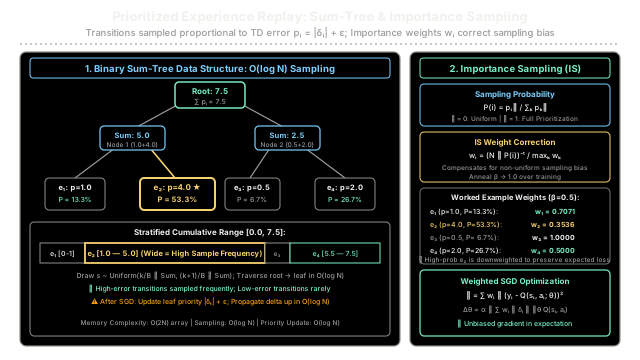
Why Does This Exist?

In standard uniform experience replay, every stored transition has an identical probability of selection:

$P(i) = \frac{1}{|\mathcal{D}|}$

In complex environments, however, transitions vary wildly in their information content. The overwhelming majority of transitions are mundane and predictable—such as driving along an empty highway or waiting in an open hallway—yielding near-zero Temporal Difference (TD) error ($|\delta| \approx 0$). In contrast, rare, critical transitions—such as colliding with an obstacle, reaching a sparse goal, or uncovering a trap—carry massive TD errors ($|\delta| \gg 0$).

Uniform replay treats these transitions as equals. A network wastes over 80% of its mini-batch compute repeatedly re-learning transitions it has already mastered, while critical bottleneck transitions may only be sampled once every tens of thousands of steps.

Introduced by Tom Schaul et al. (DeepMind, 2016), Prioritized Experience Replay (PER) replaces uniform selection by prioritizing transitions in proportion to the magnitude of their expected learning progress, proxied by their TD error $|\delta_i|$. By focusing gradient updates on transitions the current network finds most surprising, PER substantially accelerates training efficiency across challenging deep RL benchmarks.

Because non-uniform sampling fundamentally skews the state visitation distribution, PER introduces Importance Sampling (IS) weights to correct sampling bias, ensuring gradient descent converges to the true expected Bellman fixed point.

Think of It Like This

How It Actually Works

Mathematical Formulation and Sum-Tree Architecture

1. Transition Priority Metric

For transition $i = (s_i, a_i, r_i, s'_i, d_i)$, its priority $p_i$ is determined by the absolute magnitude of its TD error:

$p_i \doteq |\delta_i| + \epsilon$

Where:

• $\delta_i = r_i + \gamma (1 - d_i) \max_{a'} Q(s'_i, a'; \theta^-) - Q(s_i, a_i; \theta)$ is the TD error.
• $\epsilon > 0$ is a small positive regularization constant (e.g., $\epsilon = 10^{-5}$) ensuring that transitions with zero TD error still retain a non-zero probability of being replayed.

2. Sampling Probability Distribution

The probability of sampling transition $i$ from a buffer of size $N$ is defined by:

$P(i) \doteq \frac{p_i^\alpha}{\sum_{k=1}^N p_k^\alpha}$

Where:

• $\alpha \in [0, 1]$ dictates the degree of prioritization.
• When $\alpha = 0$, $P(i) = \frac{1}{N}$ (pure uniform sampling).
• When $\alpha = 1$, sampling is strictly proportional to priority.
• In practice, $\alpha \approx 0.6$ balances greediness against diversity.

3. Importance Sampling (IS) Bias Correction

Prioritized sampling shifts the distribution of mini-batches away from the true policy state distribution. To compensate for this bias, each sample $i$ in mini-batch $\mathcal{B}$ is weighted by an importance sampling weight $w_i$:

$w_i \doteq \left( \frac{1}{N} \cdot \frac{1}{P(i)} \right)^\beta = (N \cdot P(i))^{-\beta}$

Where $\beta \in [0, 1]$ controls the degree of bias correction. In practice, $\beta$ is annealed linearly from an initial value $\beta_0 \approx 0.4$ up to $1.0$ at the end of training. Setting $\beta = 1.0$ completely neutralizes non-uniform sampling bias.

To ensure stability and keep gradients within standard step sizes, weights are normalized by the maximum weight in the current mini-batch:

$w_i \leftarrow \frac{w_i}{\max_{k \in \mathcal{B}} w_k}$

The weighted loss minimized by gradient descent is:

$\mathcal{L}_{\text{PER}}(\theta) \doteq \frac{1}{|\mathcal{B}|} \sum_{i \in \mathcal{B}} w_i \cdot \delta_i^2$

4. The Binary Sum-Tree Data Structure

A naive implementation that calculates $P(i)$ and samples across $N = 10^6$ items requires an $O(N)$ linear pass per sample, making PER computationally intractable.

To achieve $O(\log N)$ sampling and priority updates, PER employs a Binary Sum-Tree:

• The tree is stored as a flat array of size $2N - 1$.
• The $N$ leaf nodes store the individual priorities $p_i^\alpha$.
• Each parent node stores the sum of its two children: $\text{Node}_k = \text{LeftChild} + \text{RightChild}$.
• The root node (index 0) contains the total sum of all priorities: $p_{\text{total}} = \sum_{k=1}^N p_k^\alpha$.

Stratified Sampling in $O(\log N)$: To draw a mini-batch of size $B$, the range $[0, p_{\text{total}}]$ is divided into $B$ equal segments. A value $v$ is drawn uniformly from each segment:

$v \sim \left[ \frac{k}{B} p_{\text{total}}, \frac{k+1}{B} p_{\text{total}} \right), \quad k \in \{0, \dots, B-1\}$

Starting at the root, the algorithm walks down the tree: if $v \le \text{LeftChild}$, descend left; otherwise, subtract $\text{LeftChild}$ from $v$ and descend right. A leaf is reached in exactly $\lceil \log_2 N \rceil$ comparisons.

Priority Update in $O(\log N)$: After computing new TD errors on the sampled mini-batch, each leaf's priority is updated. The change $\Delta = p_{\text{new}} - p_{\text{old}}$ propagates upward through parent pointers to the root in $O(\log N)$ operations.

Worked Numerical Example

Consider a buffer of $N = 4$ transitions with $\alpha = 1.0$, $\epsilon = 0.0$, and $\beta = 0.5$.

1. Transition Setup & Sum-Tree Construction

Four transitions arrive with the following TD error magnitudes:

• $e_1$: $|\delta_1| = 1.0 \implies p_1 = 1.0$
• $e_2$: $|\delta_2| = 4.0 \implies p_2 = 4.0$ (High TD error)
• $e_3$: $|\delta_3| = 0.5 \implies p_3 = 0.5$ (Low TD error)
• $e_4$: $|\delta_4| = 2.0 \implies p_4 = 2.0$

Total Priority: $p_{\text{total}} = 1.0 + 4.0 + 0.5 + 2.0 = 7.5$

Sum-Tree Array Structure ($2N - 1 = 7$ nodes):

• Leaf nodes (indices 3, 4, 5, 6): $\text{tree}[3] = 1.0$, $\text{tree}[4] = 4.0$, $\text{tree}[5] = 0.5$, $\text{tree}[6] = 2.0$.
• Parent of leaves 3 & 4 (index 1): $\text{tree}[1] = 1.0 + 4.0 = 5.0$.
• Parent of leaves 5 & 6 (index 2): $\text{tree}[2] = 0.5 + 2.0 = 2.5$.
• Root node (index 0): $\text{tree}[0] = 5.0 + 2.5 = 7.5$.
• Array: $[7.5, 5.0, 2.5, 1.0, 4.0, 0.5, 2.0]$.

2. Sampling Probabilities

$P(i) = \frac{p_i}{p_{\text{total}}}$

• $P(e_1) = \frac{1.0}{7.5} = \frac{2}{15} \approx 0.1333$
• $P(e_2) = \frac{4.0}{7.5} = \frac{8}{15} \approx 0.5333$ (Sampled 4x more often than $e_1$)
• $P(e_3) = \frac{0.5}{7.5} = \frac{1}{15} \approx 0.0667$
• $P(e_4) = \frac{2.0}{7.5} = \frac{4}{15} \approx 0.2667$

3. Importance Sampling Weights ($\beta = 0.5, N = 4$)

Raw weight formula: $w_i^{\text{raw}} = (4 \cdot P(i))^{-0.5} = \frac{1}{\sqrt{4 \cdot P(i)}}$:

• $e_1$: $w_1^{\text{raw}} = (4 \times 0.1333)^{-0.5} = (8/15)^{-0.5} \approx 1.3693$
• $e_2$: $w_2^{\text{raw}} = (4 \times 0.5333)^{-0.5} = (32/15)^{-0.5} \approx 0.6847$
• $e_3$: $w_3^{\text{raw}} = (4 \times 0.0667)^{-0.5} = (4/15)^{-0.5} \approx 1.9365$ ($w_{\max}$)
• $e_4$: $w_4^{\text{raw}} = (4 \times 0.2667)^{-0.5} = (16/15)^{-0.5} \approx 0.9682$

Normalize by $w_{\max} = 1.9365$:

• $w_1 = \frac{1.3693}{1.9365} = \sqrt{\frac{4}{8}} = \sqrt{0.5} \approx 0.7071$
• $w_2 = \frac{0.6847}{1.9365} = \sqrt{\frac{4}{32}} = \sqrt{0.125} \approx 0.3536$
• $w_3 = \frac{1.9365}{1.9365} = 1.0000$
• $w_4 = \frac{0.9682}{1.9365} = \sqrt{\frac{4}{16}} = 0.5000$

Notice how $e_2$, which is sampled most frequently ($P = 53.3\%$), is discounted the most ($w_2 = 0.3536$). This down-weighting prevents frequent updates on $e_2$ from dominating and destabilizing the overall gradient.

4. Post-SGD Priority Update

Suppose the network trains on $e_2$ and its TD error drops from $4.0$ to $1.0$:

• Delta: $\Delta = 1.0 - 4.0 = -3.0$.
• Leaf 4 becomes $1.0$.
• Parent node 1 becomes $5.0 + (-3.0) = 2.0$.
• Root node 0 becomes $7.5 + (-3.0) = 4.5$.
• Updated tree array: $[4.5, 2.0, 2.5, 1.0, 1.0, 0.5, 2.0]$.

The priority of $e_2$ drops automatically, naturally redirecting future sampling capacity toward remaining high-error transitions.

Code

1import math2import random3from typing import Any, List, Optional, Sequence, Tuple4
5
6class SumTree:7    """Binary Sum-Tree data structure storing priorities in leaves and sums in parents."""8
9    def __init__(self, capacity: int) -> None:10        if capacity <= 0:11            raise ValueError("Capacity must be positive.")12        self.capacity = capacity13        # Array representation of binary tree: 2 * capacity - 1 nodes14        self.tree: List[float] = [0.0] * (2 * capacity - 1)15        self.data: List[Any] = [None] * capacity16        self.write_ptr: int = 017        self.size: int = 018
19    @property20    def total_priority(self) -> float:21        """Total sum of all priorities stored at the root node."""22        return self.tree[0]23
24    def update(self, tree_idx: int, priority: float) -> None:25        """Update leaf priority and propagate change up to root in O(log N)."""26        delta = priority - self.tree[tree_idx]27        self.tree[tree_idx] = priority28
29        parent = (tree_idx - 1) // 230        while parent >= 0:31            self.tree[parent] += delta32            if parent == 0:33                break34            parent = (parent - 1) // 235
36    def add(self, priority: float, data: Any) -> int:37        """Add transition data with priority in O(log N). Overwrites oldest entry."""38        leaf_idx = self.write_ptr + self.capacity - 139        self.data[self.write_ptr] = data40        self.update(leaf_idx, priority)41
42        self.write_ptr = (self.write_ptr + 1) % self.capacity43        if self.size < self.capacity:44            self.size += 145        return leaf_idx46
47    def get(self, value: float) -> Tuple[int, float, Any]:48        """Sample leaf matching prefix sum query value in O(log N)."""49        parent = 050        while True:51            left_child = 2 * parent + 152            right_child = left_child + 153
54            if left_child >= len(self.tree):55                # Leaf reached56                leaf_idx = parent57                break58
59            if value <= self.tree[left_child]:60                parent = left_child61            else:62                value -= self.tree[left_child]63                parent = right_child64
65        data_idx = leaf_idx - self.capacity + 166        return leaf_idx, self.tree[leaf_idx], self.data[data_idx]67
68
69class PrioritizedReplayBuffer:70    """Prioritized Experience Replay buffer using a SumTree."""71
72    def __init__(73        self,74        capacity: int,75        alpha: float = 0.6,76        beta_start: float = 0.4,77        epsilon: float = 1e-5,78    ) -> None:79        self.tree = SumTree(capacity)80        self.alpha = alpha81        self.beta = beta_start82        self.epsilon = epsilon83        self.max_priority = 1.084
85    def push(self, data: Any) -> None:86        """Insert new transition with initial maximal priority."""87        priority = (self.max_priority + self.epsilon) ** self.alpha88        self.tree.add(priority, data)89
90    def sample(91        self,92        batch_size: int,93        rng: Optional[random.Random] = None,94    ) -> Tuple[List[Any], List[int], List[float]]:95        """Stratified sample of batch_size transitions with IS weights."""96        sampler = rng if rng is not None else random97        batch_data: List[Any] = []98        tree_indices: List[int] = []99        priorities: List[float] = []100
101        total_p = self.tree.total_priority102        segment_len = total_p / batch_size103
104        for i in range(batch_size):105            low = segment_len * i106            high = segment_len * (i + 1)107            query_val = sampler.uniform(low, high)108
109            leaf_idx, p, item = self.tree.get(query_val)110            tree_indices.append(leaf_idx)111            priorities.append(p)112            batch_data.append(item)113
114        # Importance sampling weights calculation115        n = self.tree.size116        probs = [p / total_p for p in priorities]117        raw_weights = [(n * prob) ** (-self.beta) for prob in probs]118        max_w = max(raw_weights) if raw_weights else 1.0119        normalized_weights = [w / max_w for w in raw_weights]120
121        return batch_data, tree_indices, normalized_weights122
123    def update_priorities(124        self, tree_indices: Sequence[int], td_errors: Sequence[float]125    ) -> None:126        """Update priorities following network gradient step."""127        for idx, error in zip(tree_indices, td_errors):128            p = (abs(error) + self.epsilon) ** self.alpha129            self.max_priority = max(self.max_priority, abs(error))130            self.tree.update(idx, p)131
132
133if __name__ == "__main__":134    # Reproduce the worked numerical example: N=4, alpha=1.0, beta=0.5, epsilon=0.0135    tree = SumTree(capacity=4)136
137    # Insert 4 items with priorities [1.0, 4.0, 0.5, 2.0]138    errors = [1.0, 4.0, 0.5, 2.0]139    for i, err in enumerate(errors):140        tree.add(priority=err, data=f"e{i+1}")141
142    total_priority = tree.total_priority143    print(f"Total Priority: {total_priority:.4f}")144    print(f"Tree Array: {[round(x, 2) for x in tree.tree]}")145
146    # Compute sampling probabilities147    probs = [err / total_priority for err in errors]148    print(f"Probabilities: {[round(p, 4) for p in probs]}")149
150    # Compute normalized IS weights (beta = 0.5, N = 4)151    beta = 0.5152    n = 4153    raw_w = [(n * p) ** (-beta) for p in probs]154    max_weight = max(raw_w)155    norm_w = [w / max_weight for w in raw_w]156    print(f"Normalized IS Weights: {[round(w, 4) for w in norm_w]}")157
158    # Test prefix sum queries159    query_vals = [0.5, 3.0, 5.2, 6.5]160    for q in query_vals:161        leaf_idx, p, item = tree.get(q)162        print(f"Query {q:3.1f} -> {item} (leaf_idx={leaf_idx}, p={p:.1f})")163
164    # Update e2 priority from 4.0 to 1.0 (leaf_idx = 4)165    print("\nUpdating e2 (leaf 4) priority from 4.0 to 1.0...")166    tree.update(4, 1.0)167    print(f"New Total Priority: {tree.total_priority:.4f}")168    print(f"Updated Tree Array: {[round(x, 2) for x in tree.tree]}")

1# Expected Output:2# Total Priority: 7.50003# Tree Array: [7.5, 5.0, 2.5, 1.0, 4.0, 0.5, 2.0]4# Probabilities: [0.1333, 0.5333, 0.0667, 0.2667]5# Normalized IS Weights: [0.7071, 0.3536, 1.0, 0.5]6# Query 0.5 -> e1 (leaf_idx=3, p=1.0)7# Query 3.0 -> e2 (leaf_idx=4, p=4.0)8# Query 5.2 -> e3 (leaf_idx=5, p=0.5)9# Query 6.5 -> e4 (leaf_idx=6, p=2.0)10# 11# Updating e2 (leaf 4) priority from 4.0 to 1.0...12# New Total Priority: 4.500013# Updated Tree Array: [4.5, 2.0, 2.5, 1.0, 1.0, 0.5, 2.0]

Watch Out For

The Quick Version

• Focuses on Surprise: Replaces uniform replay by sampling transitions proportional to their TD error ($P(i) \propto (|\delta_i| + \epsilon)^\alpha$), accelerating learning where the agent can improve the most.
• Logarithmic Complexity: Employs a binary Sum-Tree to execute non-uniform sampling and priority updates in $O(\log N)$ time, avoiding costly $O(N)$ linear scans.
• Importance Sampling Correction: Multiplies gradient steps by normalized IS weights $w_i = (N \cdot P(i))^{-\beta} / \max_k w_k$, annealing $\beta \to 1.0$ to eliminate non-uniform sampling bias.
• Prevents Lockout: Adds a small positive constant $\epsilon > 0$ to ensure zero-error transitions maintain a non-zero probability of future selection.

What to Read Next

• Experience Replay
• Deep Q-Networks
• Dueling Network Architectures