Expected SARSA

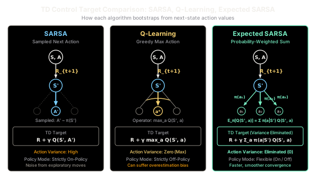
Instead of gambling on a single randomly sampled next action, Expected SARSA computes the exact average value over all available actions weighted by the probability of taking them.

Why Does This Exist?

In classical Temporal Difference learning, SARSA computes its bootstrap target using the exact action $A_{t+1}$ sampled by the agent's behavior policy:

Y_t^{\text{SARSA}} = R_{t+1} + \gamma Q(S_{t+1}, A_{t+1})

Because $A_{t+1}$ is a random draw from an exploratory policy (such as $\epsilon$ -greedy), this single sample injects massive variance into the update. Two identical transitions landing in the exact same state $S_{t+1}$ can produce wildly contradictory target values: one step samples a greedy action yielding high value, while the very next step samples an exploratory blunder yielding a catastrophic penalty. To prevent divergence from this sampling noise, practitioners must reduce the learning rate $\alpha$ , slowing convergence to a crawl.

Q-learning sidesteps this action variance by taking the greedy maximum $\max_a Q(S_{t+1}, a)$ . However, Q-learning is strictly off-policy: it assumes infallible future execution. In hazardous environments where the agent continues to explore, Q-learning ignores its own exploratory blunders, suffering from maximization bias and frequently driving the agent into catastrophic penalties during online learning.

Expected SARSA resolves this fundamental tension. Instead of rolling the dice on a single sampled action $A_{t+1}$ , it computes the exact mathematical expectation across all possible next-state actions under policy $\pi$ :

Y_t^{\text{Exp}} = R_{t+1} + \gamma \sum_{a \in \mathcal{A}} \pi(a \mid S_{t+1}) Q(S_{t+1}, a)

By replacing a random draw with its expected value, Expected SARSA completely eliminates action-selection sample variance while faithfully accounting for exploratory risk.

Think of It Like This

Calculating an exam grade: die roll vs best answer vs weighted course syllabus

Imagine a university grading policy for a multi-part final exam containing easy questions, moderate questions, and treacherous trap questions.

The SARSA examiner rolls a multi-sided die to pick a single question at random and awards you that single question's score as your entire course grade. If you roll an easy question, your recorded grade spikes; if you roll a treacherous trap question by sheer bad luck, your recorded grade plummets. Over infinite repeated exams the average score is technically correct, but every individual update suffers extreme variance from the random die roll.
The Q-learning examiner assumes you will answer only the easiest question on the entire test, completely ignoring that the exam rules force you to answer harder questions 10% of the time during testing.
The Expected SARSA examiner consults the syllabus, takes the exact probability of every question appearing, multiplies each by its expected score, and assigns your deterministic expected value: $\sum_i p_i \times \text{score}_i$ . No dice are rolled. Every evaluation is smooth, predictable, and fully accounts for the presence of the hard questions.

Where the analogy stops: A course syllabus has static question weights, whereas in reinforcement learning, both the policy distribution $\pi(a \mid s)$ and the action values $Q(s, a)$ continuously shift as the agent learns, requiring the expectation to be recomputed dynamically at every time step.

How It Actually Works

Expectation Backup and Policy Duality

Let $S_t \in \mathcal{S}$ denote the state at step $t$ , $A_t \in \mathcal{A}$ the action taken, $R_{t+1} \in \mathbb{R}$ the scalar reward, and $S_{t+1} \in \mathcal{S}$ the resulting state. The update rule for Expected SARSA is:

Q(S_t, A_t) \leftarrow Q(S_t, A_t) + \alpha \left[ R_{t+1} + \gamma \sum_{a \in \mathcal{A}} \pi(a \mid S_{t+1}) Q(S_{t+1}, a) - Q(S_t, A_t) \right]

where:

$\alpha \in (0, 1]$ is the step-size parameter (learning rate).
$\gamma \in [0, 1)$ is the discount factor.
$\pi(a \mid S_{t+1})$ is the probability of selecting action $a$ in state $S_{t+1}$ under the target policy $\pi$ .
$\sum_{a \in \mathcal{A}} \pi(a \mid S_{t+1}) Q(S_{t+1}, a) = \mathbb{E}_{\pi}[Q(S_{t+1}, \cdot)]$ is the expected action value under $\pi$ .

Variance Reduction Analysis

Consider the variance of the TD target conditioned on the transition $(S_t, A_t, R_{t+1}, S_{t+1})$ :

\text{Var}_{A_{t+1}}\left[ R_{t+1} + \gamma Q(S_{t+1}, A_{t+1}) \mid S_{t+1} \right] = \gamma^2 \text{Var}_{A_{t+1}}\left[ Q(S_{t+1}, A_{t+1}) \right]

In standard SARSA, $\text{Var}_{A_{t+1}}\left[ Q(S_{t+1}, A_{t+1}) \right] > 0$ whenever policy $\pi$ assigns non-zero probability to multiple actions with distinct values. In Expected SARSA:

\text{Var}\left[ \sum_{a} \pi(a \mid S_{t+1}) Q(S_{t+1}, a) \;\middle|\; S_{t+1} \right] = 0

The action-sampling variance is identically zero. The only remaining stochasticity in the update stems from environment dynamics (transition probabilities $P(S_{t+1} \mid S_t, A_t)$ and stochastic rewards $R_{t+1}$ ). Because variance is strictly lower, Expected SARSA can use substantially larger learning rates $\alpha$ without becoming unstable, converging faster than SARSA across almost all tabular benchmarks.

Unifying On-Policy and Off-Policy Control

Expected SARSA separates the behavior policy $b(a \mid s)$ (which selects actions in the environment) from the target policy $\pi(a \mid s)$ (which defines the expectation in the TD target):

On-Policy Expected SARSA: Set $\pi = b$ . For an $\epsilon$ -greedy policy with $|\mathcal{A}|$ actions, the greedy action $a^* = \arg\max_a Q(S_{t+1}, a)$ has probability $1 - \epsilon + \frac{\epsilon}{|\mathcal{A}|}$ , while every non-greedy action has probability $\frac{\epsilon}{|\mathcal{A}|}$ . The expectation is: $\mathbb{E}_{\pi}[Q(S_{t+1}, \cdot)] = \left(1 - \epsilon\right) \max_{a} Q(S_{t+1}, a) + \frac{\epsilon}{|\mathcal{A}|} \sum_{a \in \mathcal{A}} Q(S_{t+1}, a)$
Off-Policy (Q-learning as a special case): Set $\pi$ to be purely greedy with respect to $Q$ , assigning $\pi(a^* \mid S_{t+1}) = 1$ and $\pi(a \mid S_{t+1}) = 0$ for all $a \neq a^*$ . The expectation collapses to: $\sum_{a \in \mathcal{A}} \pi(a \mid S_{t+1}) Q(S_{t+1}, a) = \max_{a \in \mathcal{A}} Q(S_{t+1}, a)$ Expected SARSA directly reproduces Q-learning without requiring importance sampling corrections on the next action.

Worked numerical example

Let an agent be in state $S_0$ and take action $A_0 = \text{"East"}$ . The transition reaches state $S_1$ and yields immediate reward $R_{t+1} = -1.0$ .

Parameters:

Learning rate $\alpha = 0.5$
Discount factor $\gamma = 0.9$
Prior estimate $Q(S_0, \text{"East"}) = 2.0$

In state $S_1$ , there are three available actions $\mathcal{A} = \{a_1, a_2, a_3\}$ :

$a_1$ (Safe path): $Q(S_1, a_1) = 20.0$ (greedy action, $a^*$ )
$a_2$ (Detour): $Q(S_1, a_2) = 10.0$
$a_3$ (Cliff edge): $Q(S_1, a_3) = -100.0$

The agent follows an $\epsilon$ -greedy behavior policy with $\epsilon = 0.3$ :

$\pi(a_1 \mid S_1) = 1 - 0.3 + \frac{0.3}{3} = 0.7 + 0.1 = 0.8$
$\pi(a_2 \mid S_1) = \frac{0.3}{3} = 0.1$
$\pi(a_3 \mid S_1) = \frac{0.3}{3} = 0.1$

1. Expected SARSA Update

First, compute the expected next-state action value:

\mathbb{E}_\pi[Q(S_1, \cdot)] = (0.8 \times 20.0) + (0.1 \times 10.0) + (0.1 \times -100.0)

\mathbb{E}_\pi[Q(S_1, \cdot)] = 16.0 + 1.0 - 10.0 = 7.0

Compute the TD Target and error:

Y_t^{\text{Exp}} = R_{t+1} + \gamma \mathbb{E}_\pi[Q(S_1, \cdot)] = -1.0 + 0.9 \times 7.0 = -1.0 + 6.3 = 5.3

\delta_t^{\text{Exp}} = 5.3 - Q(S_0, A_0) = 5.3 - 2.0 = 3.3

Update the Q-value:

Q(S_0, A_0) \leftarrow 2.0 + 0.5 \times 3.3 = 2.0 + 1.65 = 3.65

2. Contrast with SARSA (Sample-Dependent)

Case A (Agent randomly samples greedy action $a_1$ ): $Y_t^{\text{SARSA}} = -1.0 + 0.9 \times 20.0 = 17.0 \implies \delta_t = 15.0$ $Q(S_0, A_0) \leftarrow 2.0 + 0.5 \times 15.0 = 9.5$
Case B (Agent randomly samples cliff blunder $a_3$ ): $Y_t^{\text{SARSA}} = -1.0 + 0.9 \times (-100.0) = -91.0 \implies \delta_t = -93.0$ $Q(S_0, A_0) \leftarrow 2.0 + 0.5 \times (-93.0) = -44.5$

3. Contrast with Q-Learning (Greedy Max)

Y_t^{\text{Q}} = -1.0 + 0.9 \times \max(20.0, 10.0, -100.0) = -1.0 + 0.9 \times 20.0 = 17.0

Q(S_0, A_0) \leftarrow 2.0 + 0.5 \times (17.0 - 2.0) = 9.5

Key Takeaway: SARSA's estimate oscillates violently between $+9.5$ and $-44.5$ based entirely on the roll of the exploration dice. Q-learning blindly assumes future perfection ( $+9.5$ ), ignoring that the agent falls off the cliff 10% of the time. Expected SARSA produces a steady, deterministic update ( $3.65$ ), accurately penalizing the cliff risk without sample variance.

Code

1from typing import Dict, List2import numpy as np3
4def compute_epsilon_greedy_probs(5    q_values: np.ndarray,6    epsilon: float,7) -> np.ndarray:8    """Computes action probabilities under an epsilon-greedy policy."""9    num_actions = len(q_values)10    best_action = int(np.argmax(q_values))11    probs = np.full(num_actions, epsilon / num_actions, dtype=np.float64)12    probs[best_action] += 1.0 - epsilon13    return probs14
15def step_expected_sarsa(16    q_table: Dict[str, np.ndarray],17    s: str,18    a_idx: int,19    r: float,20    s_next: str,21    target_probs: np.ndarray,22    alpha: float = 0.5,23    gamma: float = 0.9,24) -> float:25    """Updates Q-table using Expected SARSA probability-weighted target."""26    expected_next_q = float(np.dot(target_probs, q_table[s_next]))27    target = r + gamma * expected_next_q28    td_error = target - q_table[s][a_idx]29    q_table[s][a_idx] += alpha * td_error30    return float(q_table[s][a_idx])31
32def step_sarsa(33    q_table: Dict[str, np.ndarray],34    s: str,35    a_idx: int,36    r: float,37    s_next: str,38    a_next_idx: int,39    alpha: float = 0.5,40    gamma: float = 0.9,41) -> float:42    """Updates Q-table using standard SARSA sampled-action target."""43    target = r + gamma * float(q_table[s_next][a_next_idx])44    td_error = target - q_table[s][a_idx]45    q_table[s][a_idx] += alpha * td_error46    return float(q_table[s][a_idx])47
48def step_q_learning(49    q_table: Dict[str, np.ndarray],50    s: str,51    a_idx: int,52    r: float,53    s_next: str,54    alpha: float = 0.5,55    gamma: float = 0.9,56) -> float:57    """Updates Q-table using Q-learning greedy max target."""58    target = r + gamma * float(np.max(q_table[s_next]))59    td_error = target - q_table[s][a_idx]60    q_table[s][a_idx] += alpha * td_error61    return float(q_table[s][a_idx])62
63# Environment setup matching the worked numerical example64# S1 actions: [Safe path = 20.0, Detour = 10.0, Cliff edge = -100.0]65q_exp = {"S0": np.array([2.0]), "S1": np.array([20.0, 10.0, -100.0])}66q_sarsa_safe = {"S0": np.array([2.0]), "S1": np.array([20.0, 10.0, -100.0])}67q_sarsa_cliff = {"S0": np.array([2.0]), "S1": np.array([20.0, 10.0, -100.0])}68q_ql = {"S0": np.array([2.0]), "S1": np.array([20.0, 10.0, -100.0])}69
70# Target policy: epsilon-greedy with epsilon = 0.3 -> probs = [0.8, 0.1, 0.1]71probs = compute_epsilon_greedy_probs(q_exp["S1"], epsilon=0.3)72
73# 1. Expected SARSA update74val_exp = step_expected_sarsa(q_exp, "S0", 0, -1.0, "S1", probs)75
76# 2. SARSA updates: sampled greedy (index 0) vs sampled blunder (index 2)77val_sarsa_safe = step_sarsa(q_sarsa_safe, "S0", 0, -1.0, "S1", a_next_idx=0)78val_sarsa_cliff = step_sarsa(q_sarsa_cliff, "S0", 0, -1.0, "S1", a_next_idx=2)79
80# 3. Q-learning update (greedy max)81val_ql = step_q_learning(q_ql, "S0", 0, -1.0, "S1")82
83print(f"Expected SARSA Q(S0, East): {val_exp:.2f}")84# -> Expected SARSA Q(S0, East): 3.6585
86print(f"SARSA (sampled safe) Q(S0, East): {val_sarsa_safe:.2f}")87# -> SARSA (sampled safe) Q(S0, East): 9.5088
89print(f"SARSA (sampled cliff) Q(S0, East): {val_sarsa_cliff:.2f}")90# -> SARSA (sampled cliff) Q(S0, East): -44.5091
92print(f"Q-learning Q(S0, East): {val_ql:.2f}")93# -> Q-learning Q(S0, East): 9.50

Watch Out For

Computational Bottleneck When Action Space |A| Is Massive

While standard SARSA performs an $O(1)$ array lookup for the sampled action $A_{t+1}$ and Q-learning requires an $O(|\mathcal{A}|)$ maximum, Expected SARSA must evaluate the full dot product $\sum_{a \in \mathcal{A}} \pi(a \mid S_{t+1}) Q(S_{t+1}, a)$ across all actions on every transition.

For small action spaces (such as gridworlds or standard discrete control tasks with 4 to 20 actions), this dot product is trivial and the variance reduction yields immediate wall-clock speedups. However, in recommender systems or combinatorial control environments with hundreds of thousands of discrete actions, calculating the explicit expectation at every step creates a severe computational bottleneck. Furthermore, in continuous action spaces, computing the integral $\int \pi(a \mid s) Q(s, a) da$ analytically is intractable without specialized parameterizations.

Concrete Fix:

Under $\epsilon$ -greedy policies, avoid generating the full probability vector. Decompose the expectation into greedy and uniform components: $\mathbb{E}_\pi[Q] = (1 - \epsilon)\max_a Q + \frac{\epsilon}{|\mathcal{A}|}\sum_a Q$ , which can be computed in a single vectorized pass.
For massive action spaces, use Sampled Expected SARSA: approximate the expectation using a mini-batch of $K \ll |\mathcal{A}|$ sampled actions, capturing most variance-reduction benefits at a fraction of the computational cost.

The Quick Version

Expected SARSA replaces the single sampled next action $Q(S_{t+1}, A_{t+1})$ with the policy-weighted expectation $\sum_a \pi(a \mid S_{t+1}) Q(S_{t+1}, a)$ .
Eliminating action-selection sample variance allows Expected SARSA to train stably with significantly higher learning rates $\alpha$ than standard SARSA.
Expected SARSA smoothly unifies on-policy and off-policy TD learning: setting the target policy to the greedy policy reproduces Q-learning without importance sampling corrections.
The primary trade-off is computational: evaluating the expectation requires an inner product over $|\mathcal{A}|$ actions at every step, making it ideal for discrete spaces but requiring approximations for massive or continuous action domains.