Experience Replay

Experience replay stores past transitions in a circular memory buffer and samples random mini-batches, breaking temporal correlations for stable deep neural network training.

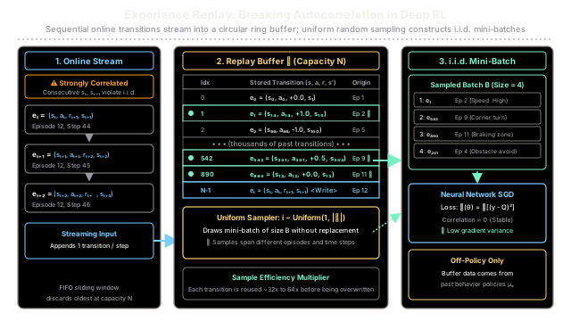
Why Does This Exist?

When researchers first attempted to combine reinforcement learning with deep neural networks in the early 2010s, training routinely collapsed. Value estimates fluctuated wildly, gradients exploded or vanished, and agents failed to solve even rudimentary Atari titles.

This failure stemmed from two fundamental obstacles inherent to sequential decision-making:

Severe Temporal Autocorrelation: Standard stochastic gradient descent (SGD) algorithms rely on the foundational assumption that training samples are independent and identically distributed (i.i.d.). In reinforcement learning, however, the agent collects data sequentially: state $S_{t+1}$ strongly depends on state $S_t$ . If a car simulator spends 30 seconds navigating an open highway, every consecutive gradient update trains the network exclusively on high-speed straightaways. When the car eventually encounters a sharp curve, the network has overwritten its cornering weights—a pathology known as catastrophic forgetting.
Extreme Sample Inefficiency: Physical robot actuators wear out, and complex game engines run at bounded frame rates. In standard online reinforcement learning, a transition $(s_t, a_t, r_{t+1}, s_{t+1})$ is used for a single gradient step and instantly discarded. Discarding hard-won experience after one update wastes critical training signal.

Originally proposed by Long-Ji Lin (1992) and revitalized by Mnih et al. (2015) in the landmark Deep Q-Network (DQN) paper, Experience Replay solves both dilemmas simultaneously. By storing transitions in a circular sliding buffer $\mathcal{D}$ and drawing randomized mini-batches for optimization, experience replay breaks temporal correlations, restores approximate i.i.d. conditions, and reuses each transition dozens of times across training.

Think of It Like This

The Basketball Film Review Session

Imagine an NBA basketball player working to improve their court decision-making.

If the player trained without experience replay (pure online streaming), they would evaluate their gameplay strictly play-by-play in real time. If they just missed a contested three-pointer on a fast break, they would spend the next five minutes obsessing exclusively over their three-point shooting mechanics. In doing so, they would neglect defensive rebounding, pick-and-roll defense, and passing vision. The latest event would dictate all immediate learning, leading to erratic performance swings.

With experience replay, the coaching staff instead records every possession throughout the season into an indexed video archive. During training film sessions, the coaching staff shuffles and selects a randomized review reel of five plays:

A fast-break turnover from three weeks ago
A successful defensive box-out from last night
A baseline inbound pass against a zone defense from two months ago
A clutch free throw under pressure
A transition foul from yesterday's second quarter

Because the film session mixes diverse situations across different opponents and game quarters, the player develops robust, balanced habits rather than overreacting to the single play they executed five seconds ago.

Where the analogy stops: Human coaches deliberately bias film sessions toward critical mistakes (analogous to Prioritized Experience Replay). In standard uniform experience replay, every transition in the sliding memory buffer has an equal probability of selection, regardless of whether the agent succeeded, failed, or was surprised.

How It Actually Works

Mathematical Formulation and Buffer Mechanics

At each time step $t$ , the agent interacts with the environment by executing action $a_t$ in state $s_t$ , receiving scalar reward $r_{t+1}$ , transitioning to next state $s_{t+1}$ , and observing a boolean termination flag $d_{t+1} \in \{0, 1\}$ . This interaction forms a transition tuple:

$e_t \doteq (s_t, a_t, r_{t+1}, s_{t+1}, d_{t+1})$

The agent appends $e_t$ to a fixed-capacity replay dataset:

$\mathcal{D} = \{ e_1, e_2, \dots, e_{|\mathcal{D}|} \}, \quad |\mathcal{D}| \le N$

Where $N$ is the maximum buffer capacity (typically $N \in [10^5, 10^6]$ in deep RL).

Circular Ring Buffer (FIFO) Logic

Memory is allocated as a circular queue of fixed size $N$ . When the buffer reaches full capacity ( $|\mathcal{D}| = N$ ), incoming transitions overwrite the oldest stored entries at index:

$\text{index} = t \pmod N$

Uniform Mini-Batch Sampling

During gradient optimization, the agent draws a mini-batch $\mathcal{B}$ of size $B$ (commonly $B = 32, 64, \text{ or } 256$ ) uniformly at random from $\mathcal{D}$ :

$e^{(i)} \sim \text{Uniform}(\mathcal{D}), \quad P(e^{(i)} = e_k) = \frac{1}{|\mathcal{D}|}, \quad \forall k \in \{1, \dots, |\mathcal{D}|\}$

The deep Q-learning loss over mini-batch $\mathcal{B}$ is formulated as:

$\mathcal{L}(\theta) \doteq \frac{1}{B} \sum_{i=1}^B \left( y^{(i)} - Q(s^{(i)}, a^{(i)}; \theta) \right)^2$

Where the target $y^{(i)}$ is computed using a semi-static target network $\theta^-$ :

$y^{(i)} \doteq r^{(i)} + \gamma (1 - d^{(i)}) \max_{a'} Q(s'^{(i)}, a'; \theta^-)$

The Variance Reduction Mechanism

Why does uniform sampling stabilize training? Consider estimating the expected gradient $\mathbf{g} = \mathbb{E}[\nabla_\theta \mathcal{L}]$ using a mini-batch of size $B$ . If the samples in the batch exhibit temporal autocorrelation with lag- $k$ correlation coefficients $\rho_k$ , the variance of the mini-batch gradient estimator satisfies:

$\operatorname{Var}\left( \frac{1}{B} \sum_{i=1}^B \mathbf{g}_i \right) = \frac{\sigma^2}{B} \left[ 1 + 2 \sum_{k=1}^{B-1} \left(1 - \frac{k}{B}\right) \rho_k \right]$

In sequential online streams, consecutive states often yield $\rho_1 \approx 0.8$ to $0.99$ , drastically inflating gradient variance and reducing the effective batch size. By sampling uniformly across thousands of historical episodes, the inter-sample correlation drops to zero ( $\rho_k \to 0$ ), collapsing the variance multiplier to $1$ and restoring standard SGD convergence properties.

The Off-Policy Prerequisite

Because the replay buffer stores transitions collected thousands of environment steps in the past, those transitions were generated by previous parameter configurations $\theta_{t-k}$ (historical behavior policies $b$ ).

Consequently, experience replay can only be deployed with off-policy algorithms (such as Q-Learning, DQN, DDPG, TD3, and SAC) whose value objectives evaluate target policy $\pi$ while learning from arbitrary behavior distributions $b$ . Standard on-policy methods (like REINFORCE, A2C, or vanilla PPO) cannot use experience replay without importance sampling corrections.

Worked Numerical Example

To understand the mechanics, consider a compact circular replay buffer with capacity $N = 4$ and a mini-batch size $B = 2$ .

Step 1: Sequential Insertion and Buffer Wrap-Around

The agent collects 5 transitions over time:

$t=1$ : $e_1 = (s=1.0, a=0, r=0.0, s'=2.0, d=0)$ $\to$ Stored at slot 0. Buffer: $[e_1]$ , size=1, ptr=1.
$t=2$ : $e_2 = (s=2.0, a=1, r=1.0, s'=3.0, d=0)$ $\to$ Stored at slot 1. Buffer: $[e_1, e_2]$ , size=2, ptr=2.
$t=3$ : $e_3 = (s=3.0, a=0, r=0.0, s'=4.0, d=0)$ $\to$ Stored at slot 2. Buffer: $[e_1, e_2, e_3]$ , size=3, ptr=3.
$t=4$ : $e_4 = (s=4.0, a=1, r=2.0, s'=5.0, d=1)$ $\to$ Stored at slot 3. Buffer: $[e_1, e_2, e_3, e_4]$ , size=4 (Full), ptr=0.
$t=5$ : $e_5 = (s=10.0, a=0, r=0.5, s'=11.0, d=0)$ $\to$ Overwrites slot 0!

Buffer contents at $t=5$ :

Slot 0: $e_5 = (10.0, 0, 0.5, 11.0, \text{False})$
Slot 1: $e_2 = (2.0, 1, 1.0, 3.0, \text{False})$
Slot 2: $e_3 = (3.0, 0, 0.0, 4.0, \text{False})$
Slot 3: $e_4 = (4.0, 1, 2.0, 5.0, \text{True})$
Write pointer: index 1.

Step 2: Mini-Batch Sampling

The uniform sampler draws a mini-batch of size $B = 2$ : $\mathcal{B} = [e_2, e_5]$

Notice how $e_2$ originated from an early trajectory step ( $s=2.0$ ) while $e_5$ originated from a completely different high-magnitude state ( $s=10.0$ ). The mini-batch breaks the sequential chain.

Step 3: Q-Learning Loss Calculation

Let the Q-function be a linear parameterized model: $Q(s, a; \mathbf{w}) = w_a \cdot s$ .

Current parameters: $w_0 = 0.5, w_1 = 0.5$ .
Target network parameters: identical ( $w_0^- = 0.5, w_1^- = 0.5$ ).
Discount factor: $\gamma = 0.9$ .

Processing Transition $e_2$ ( $s=2.0, a=1, r=1.0, s'=3.0, d=0$ ):

Next state values: $Q(3.0, 0; \mathbf{w}^-) = 0.5 \times 3.0 = 1.5, \quad Q(3.0, 1; \mathbf{w}^-) = 0.5 \times 3.0 = 1.5$
Target: $y_2 = r + \gamma (1 - d) \max_{a'} Q(3.0, a'; \mathbf{w}^-) = 1.0 + 0.9(1 - 0)(1.5) = 1.0 + 1.35 = 2.3500$
Prediction: $Q(2.0, 1; \mathbf{w}) = w_1 \times 2.0 = 0.5 \times 2.0 = 1.0000$
Prediction error: $\delta_2 = y_2 - Q(2.0, 1; \mathbf{w}) = 2.3500 - 1.0000 = 1.3500$

Processing Transition $e_5$ ( $s=10.0, a=0, r=0.5, s'=11.0, d=0$ ):

Next state values: $Q(11.0, 0; \mathbf{w}^-) = 0.5 \times 11.0 = 5.5, \quad Q(11.0, 1; \mathbf{w}^-) = 0.5 \times 11.0 = 5.5$
Target: $y_5 = r + \gamma (1 - d) \max_{a'} Q(11.0, a'; \mathbf{w}^-) = 0.5 + 0.9(1 - 0)(5.5) = 0.5 + 4.95 = 5.4500$
Prediction: $Q(10.0, 0; \mathbf{w}) = w_0 \times 10.0 = 0.5 \times 10.0 = 5.0000$
Prediction error: $\delta_5 = y_5 - Q(10.0, 0; \mathbf{w}) = 5.4500 - 5.0000 = 0.4500$

Mini-Batch Mean Squared Error Loss: $\mathcal{L} = \frac{1}{2} \left( \delta_2^2 + \delta_5^2 \right) = \frac{1}{2} \left( 1.3500^2 + 0.4500^2 \right) = \frac{1}{2} (1.8225 + 0.2025) = 1.0125$

Code

1import random2from typing import List, NamedTuple, Optional, Sequence, Tuple3
4
5class Transition(NamedTuple):6    """Represents an atomic environment interaction tuple."""7
8    state: float9    action: int10    reward: float11    next_state: float12    done: bool13
14
15class CircularReplayBuffer:16    """Fixed-capacity circular ring buffer with uniform mini-batch sampling."""17
18    def __init__(self, capacity: int) -> None:19        if capacity <= 0:20            raise ValueError("Buffer capacity must be positive.")21        self.capacity = capacity22        self.buffer: List[Transition] = []23        self.position: int = 024
25    def push(26        self,27        state: float,28        action: int,29        reward: float,30        next_state: float,31        done: bool,32    ) -> None:33        """Store a transition tuple. Overwrites oldest entry when buffer is full."""34        transition = Transition(state, action, reward, next_state, done)35        if len(self.buffer) < self.capacity:36            self.buffer.append(transition)37        else:38            self.buffer[self.position] = transition39
40        # Advance circular pointer41        self.position = (self.position + 1) % self.capacity42
43    def sample(44        self,45        batch_size: int,46        rng: Optional[random.Random] = None,47    ) -> List[Transition]:48        """Draw a uniform random mini-batch without replacement."""49        if len(self.buffer) < batch_size:50            raise ValueError(51                f"Cannot sample {batch_size} items from buffer of size {len(self.buffer)}."52            )53        sampler = rng if rng is not None else random54        return sampler.sample(self.buffer, batch_size)55
56    def __len__(self) -> int:57        return len(self.buffer)58
59
60def compute_mini_batch_loss(61    batch: Sequence[Transition],62    weights: Sequence[float],63    target_weights: Sequence[float],64    gamma: float = 0.9,65) -> Tuple[float, List[float]]:66    """Compute MSE loss and TD errors for a linear Q-function: Q(s, a) = w[a] * s."""67    squared_errors: List[float] = []68    td_errors: List[float] = []69
70    for t in batch:71        # Target network values: max_a' Q(s', a'; w^-)72        q_next_max = max(w * t.next_state for w in target_weights)73        target = t.reward + (0.0 if t.done else gamma * q_next_max)74
75        # Current network prediction: Q(s, a; w)76        prediction = weights[t.action] * t.state77        delta = target - prediction78
79        td_errors.append(delta)80        squared_errors.append(delta**2)81
82    mse_loss = sum(squared_errors) / len(batch)83    return mse_loss, td_errors84
85
86if __name__ == "__main__":87    # 1. Initialize buffer of capacity 488    replay_buffer = CircularReplayBuffer(capacity=4)89
90    # 2. Add 5 transitions (e5 overwrites e1 at slot 0)91    transitions_to_push = [92        (1.0, 0, 0.0, 2.0, False),  # e193        (2.0, 1, 1.0, 3.0, False),  # e294        (3.0, 0, 0.0, 4.0, False),  # e395        (4.0, 1, 2.0, 5.0, True),  # e496        (10.0, 0, 0.5, 11.0, False),  # e5 -> overwrites slot 097    ]98
99    for item in transitions_to_push:100        replay_buffer.push(*item)101
102    print(f"Buffer Capacity: {replay_buffer.capacity}, Current Size: {len(replay_buffer)}")103    print(f"Next write pointer position: {replay_buffer.position}")104
105    # Inspect current slots106    for idx, trans in enumerate(replay_buffer.buffer):107        print(f"  Slot {idx}: state={trans.state:4.1f}, action={trans.action}, r={trans.reward:3.1f}")108
109    # 3. Deterministically evaluate the batch [e2, e5] (slots 1 and 0)110    sample_batch = [replay_buffer.buffer[1], replay_buffer.buffer[0]]111    w = [0.5, 0.5]112    w_target = [0.5, 0.5]113
114    loss, errors = compute_mini_batch_loss(sample_batch, w, w_target, gamma=0.9)115
116    print(f"\nSampled Batch Transitions: e2 (state={sample_batch[0].state}), e5 (state={sample_batch[1].state})")117    print(f"TD Error e2: {errors[0]:.4f}")118    print(f"TD Error e5: {errors[1]:.4f}")119    print(f"Mini-Batch MSE Loss: {loss:.4f}")

1# Expected Output:2# Buffer Capacity: 4, Current Size: 43# Next write pointer position: 14#   Slot 0: state=10.0, action=0, r=0.55#   Slot 1: state= 2.0, action=1, r=1.06#   Slot 2: state= 3.0, action=0, r=0.07#   Slot 3: state= 4.0, action=1, r=2.08# 9# Sampled Batch Transitions: e2 (state=2.0), e5 (state=10.0)10# TD Error e2: 1.350011# TD Error e5: 0.450012# Mini-Batch MSE Loss: 1.0125

Watch Out For

The On-Policy Incompatibility and Buffer Staleness Trap

Practitioners commonly commit two major architectural errors when using experience replay:

Deploying Replay with On-Policy Algorithms: Attempting to feed replay buffer transitions into on-policy algorithms (such as PPO, A2C, or SARSA) violates policy evaluation assumptions. Because transitions stored in $\mathcal{D}$ were generated by previous policy checkpoints ( $\pi_{\theta_{t-k}}$ ), they reflect an outdated state distribution. Applying on-policy policy gradient formulas directly to stale transitions causes uncontrolled policy drift and rapid collapse.
Improper Buffer Capacity Sizing:

Buffer too small ( $N < 10^4$ ): The buffer fails to decorrelate samples. The agent suffers from catastrophic forgetting, cycling through local policies without acquiring global mastery.
Buffer too large ( $N > 10^7$ ): The buffer retains vast quantities of poor-quality exploratory transitions collected early in training when the policy was effectively random. Stale low-reward data dilutes recent high-performing demonstrations, dramatically slowing convergence.

The Fix: Use experience replay strictly with off-policy algorithms (DQN, DDPG, TD3, SAC). Calibrate buffer capacity to balance diversity against policy freshness (typically $N \in [10^5, 10^6]$ for continuous control or Atari). If high-value transitions are rare, upgrade from uniform sampling to Prioritized Experience Replay (PER) using importance sampling corrections.

The Quick Version

Decorrelates Observations: Shuffles sequential environment interactions, breaking severe temporal autocorrelation and restoring the i.i.d. conditions required by gradient descent.
Amplifies Sample Efficiency: Stores transitions in a fixed-size FIFO circular buffer, allowing each expensive environment interaction to be reused across dozens of mini-batch gradient updates.
Strictly Off-Policy: Because buffered transitions reflect historical policy checkpoints, experience replay can only be used with off-policy value-based or actor-critic methods.
Capacity Balancing: Sizing the buffer requires trading off catastrophic forgetting (buffer too small) against training on obsolete, stale exploration data (buffer too large).