Fundamentals of Reinforcement Learning

Reinforcement learning is learning what to do by trial and error—an agent interacts with an environment, receiving rewards or penalties, to discover actions that maximize long-term return.

The agent-environment loop formalizes trial-and-error learning, where an agent observes states, executes actions, and receives delayed rewards to maximize cumulative return.

Why Does This Exist?

In supervised learning, an external teacher provides explicit ground-truth labels for every input. If you train a vision model to recognize traffic signs, each image comes pre-packaged with the correct category. But in real-world sequential decision-making—controlling an autonomous vehicle, balancing a power grid, or mastering chess—no supervisor stands by to tell the system the exact optimal motor voltage or steering angle at every microsecond.

When an agent acts sequentially, three distinct hurdles emerge that supervised and unsupervised methods cannot address:

Evaluative feedback instead of instructive labels: The environment does not tell the agent what the best action would have been. It only provides a scalar score indicating how well the chosen action turned out.
Delayed consequences: An action taken at the beginning of an episode may directly trigger a catastrophe or victory fifty time steps later. Optimizing solely for immediate gain leads to disastrous traps.
Active data distribution: Unlike static dataset training where examples are independent and identically distributed (i.i.d.), the agent's current policy directly determines which future states it will visit. Poor early choices cascade into unfamiliar situations.

Reinforcement learning (RL) exists to solve this problem: it formalizes how an autonomous agent can learn goal-directed behavior purely from trial, error, and delayed reward signals.

Think of It Like This

Training a puppy with treats and timing

Imagine training an eight-week-old puppy to sit on command. You cannot hand the puppy an anatomy diagram or verbally explain the biomechanics of bending its hind legs.

Instead, the puppy is the agent, and your living room is the environment. The puppy's current posture and your vocal command constitute the state $S_t$ . The puppy experiments with various actions $A_t$ —it jumps, sniffs your shoe, wanders off, or bends its knees.

When its hindquarters finally touch the floor, you immediately deliver a tasty liver treat—the reward $R_{t+1}$ . The puppy does not know calculus, but over repeated trials, it updates its internal behavioral strategy (its policy $\pi$ ) to associate sitting with high cumulative reward.

Crucially, consider what happens if you delay the treat by twenty seconds. During those twenty seconds, the puppy stands back up, barks at the window, and chews on the carpet. If you hand over the treat then, the puppy assumes it is being rewarded for chewing the carpet. This is the temporal credit assignment problem: assigning reward to the specific prior action that actually earned it.

Where the analogy stops: Real puppies possess evolutionary instincts, fatigue, emotional attachment, and biological survival drives. A mathematical RL agent possesses none of these—it optimizes strictly and literally for the mathematical sum of the reward function you define, cheerfully exploiting every unintended loophole.

How It Actually Works

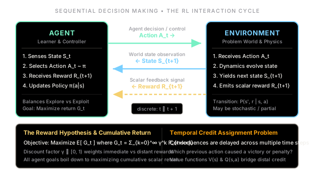
The agent-environment interaction loop

Reinforcement learning formalizes sequential decision making as a closed loop between an agent (the learner and decision-maker) and an environment (everything outside the agent).

The interaction unfolds across a sequence of discrete time steps $t = 0, 1, 2, \dots$ :

At time step $t$ , the agent senses the environment's current state $S_t \in \mathcal{S}$ , where $\mathcal{S}$ is the set of all valid states.
Based on this state, the agent selects an action $A_t \in \mathcal{A}(S_t)$ according to its policy $\pi$ : $\pi(a \mid s) = P(A_t = a \mid S_t = s)$
The environment receives $A_t$ $A_{t}$ , updates its internal dynamics, and responds at step $t+1$ $t + 1$ with two signals:
- A scalar reward $R_{t+1} \in \mathbb{R}$ .
- A subsequent state $S_{t+1} \in \mathcal{S}$ .

This transition is governed by the environment dynamics function: $p(s', r \mid s, a) = P(S_{t+1} = s', R_{t+1} = r \mid S_t = s, A_t = a)$

This cycle produces an ongoing trajectory of experience: $\tau = (S_0, A_0, R_1, S_1, A_1, R_2, S_2, \dots)$

The reward hypothesis and cumulative return

The core premise of reinforcement learning is encapsulated in Richard Sutton's Reward Hypothesis:

All of what we mean by goals and purposes can be well thought of as the maximization of the expected value of the cumulative sum of a received scalar signal (called reward).

The agent's objective is never to maximize just the immediate reward $R_{t+1}$ , but the expected cumulative return $G_t$ received from time step $t$ forward. For continuing tasks that do not naturally terminate, an unweighted infinite sum could diverge to infinity. RL introduces a discount factor $\gamma \in [0, 1)$ to ensure mathematical convergence and reflect temporal preference:

$G_t = \sum_{k=0}^{\infty} \gamma^k R_{t+k+1} = R_{t+1} + \gamma R_{t+2} + \gamma^2 R_{t+3} + \dots$

The discount factor controls the agent's temporal horizon:

When $\gamma = 0$ , the agent is purely myopic, optimizing solely for the immediate reward $R_{t+1}$ .
As $\gamma \to 1$ , the agent becomes increasingly far-sighted, giving substantial weight to rewards far into the future.

Returns obey a fundamental recursive relationship: $G_t = R_{t+1} + \gamma G_{t+1}$

The temporal credit assignment problem

Because rewards can be delayed by dozens or hundreds of steps, the agent faces the challenge of temporal credit assignment: identifying which past decisions were responsible for a distant reward or penalty.

To solve this, RL algorithms estimate value functions that quantify the long-term return expected from a given situation:

State-Value Function $V^\pi(s)$ : Expected return starting from state $s$ under policy $\pi$ : $V^\pi(s) = \mathbb{E}_\pi \left[ G_t \mid S_t = s \right]$
Action-Value Function $Q^\pi(s, a)$ : Expected return starting from state $s$ , taking action $a$ , and subsequently following $\pi$ : $Q^\pi(s, a) = \mathbb{E}_\pi \left[ G_t \mid S_t = s, A_t = a \right]$

Value functions act as an internal scorekeeper, propagating distant rewards backwards so the agent can make forward-looking choices at every step.

Worked numerical example

Consider an agent navigating a short path with discount factor $\gamma = 0.90$ . The episode runs for 3 discrete time steps until reaching a terminal state:

Time $t=0$ : Agent starts at $S_0 = \text{Start}$ . Chooses action $A_0 = \text{Advance}$ .
Environment emits immediate reward $R_1 = 0.0$ and transitions to $S_1 = \text{Corridor}$ .
Time $t=1$ : Agent at $S_1$ . Chooses action $A_1 = \text{Cross Rough Terrain}$ .
Environment emits immediate penalty $R_2 = -2.0$ (energy cost) and transitions to $S_2 = \text{Goal Approach}$ .
Time $t=2$ : Agent at $S_2$ . Chooses action $A_2 = \text{Enter Goal}$ .
Environment emits terminal goal reward $R_3 = +10.0$ and transitions to terminal state $S_3 = \text{Goal}$ .

We calculate the realized return $G_t$ at each step by working backwards from the end of the episode:

Return at $t=2$ : $G_2 = R_3 = 10.00$
Return at $t=1$ : $G_1 = R_2 + \gamma G_2 = -2.00 + 0.90 \times (10.00) = -2.00 + 9.00 = +7.00$
Return at $t=0$ : $G_0 = R_1 + \gamma G_1 = 0.00 + 0.90 \times (7.00) = 0.00 + 6.30 = +6.30$

We can verify $G_0$ by summing directly from the definition: $G_0 = R_1 + \gamma R_2 + \gamma^2 R_3 = 0.0 + 0.90 \times (-2.0) + (0.90)^2 \times (10.0) = -1.80 + 0.81 \times 10.0 = +6.30$

The myopic trap comparison

Now contrast this with a short-sighted agent that considers only immediate reward ( $\gamma = 0$ ). At $t=0$ , this agent chooses an alternative action $A_0' = \text{Take Snack}$ offering immediate reward $R_1' = +1.50$ , but leading into a dead-end swamp state where subsequent rewards are $R_2' = -5.00$ and $R_3' = 0.00$ :

$G_0^{\text{trap}} = R_1' + \gamma R_2' + \gamma^2 R_3' = 1.50 + 0.90(-5.00) + (0.90)^2(0.00) = 1.50 - 4.50 = -3.00$

While the greedy agent seemed ahead after step 1 ( $+1.50$ vs $0.00$ ), the long-term RL agent achieves a net return of $+6.30$ versus $-3.00$ . Optimizing cumulative return $G_t$ prevents the agent from walking into immediate-gratification traps.

Code

Below is a self-contained Python implementation of a 1D discrete environment that demonstrates the agent-environment step loop, transition tracking, and recursive discounted return calculation.

1from dataclasses import dataclass2from typing import List, Tuple3
4
5@dataclass6class Transition:7    """Represents a single step transition (S_t, A_t, R_{t+1}, S_{t+1}, done)."""8    state: int9    action: int10    reward: float11    next_state: int12    done: bool13
14
15class Simple1DGridWorld:16    """A 1D environment with 5 states: [0: Trap, 1, 2: Start, 3, 4: Goal].17    18    Actions:19      0 = Move Left (-1)20      1 = Move Right (+1)21    """22
23    def __init__(self, size: int = 5, goal: int = 4, trap: int = 0) -> None:24        self.size = size25        self.goal = goal26        self.trap = trap27        self.state = 2  # default center start28
29    def reset(self, start_state: int = 2) -> int:30        """Resets the environment to initial state S_0."""31        self.state = start_state32        return self.state33
34    def step(self, action: int) -> Tuple[int, float, bool]:35        """Executes action A_t, returning (S_{t+1}, R_{t+1}, done)."""36        step_delta = -1 if action == 0 else 137        self.state = max(0, min(self.size - 1, self.state + step_delta))38
39        if self.state == self.goal:40            return self.state, 10.0, True41        elif self.state == self.trap:42            return self.state, -5.0, True43        else:44            return self.state, -0.1, False45
46
47def compute_discounted_returns(48    transitions: List[Transition], gamma: float = 0.9049) -> List[float]:50    """Computes G_t backwards using the recursive relation: G_t = R_{t+1} + gamma * G_{t+1}."""51    returns: List[float] = [0.0] * len(transitions)52    running_return = 0.053
54    for t in reversed(range(len(transitions))):55        running_return = transitions[t].reward + gamma * running_return56        returns[t] = round(running_return, 4)57
58    return returns59
60
61if __name__ == "__main__":62    env = Simple1DGridWorld()63    gamma = 0.9064
65    # Execute a forward policy: move right twice from state 2 to reach goal 466    current_state = env.reset(start_state=2)67    actions = [1, 1]  # Right, Right68    episode_history: List[Transition] = []69
70    print(f"Initial State S_0: {current_state}")71    print("-" * 55)72
73    for step_idx, action in enumerate(actions):74        next_state, reward, done = env.step(action)75        transition = Transition(76            state=current_state,77            action=action,78            reward=reward,79            next_state=next_state,80            done=done,81        )82        episode_history.append(transition)83        current_state = next_state84        if done:85            break86
87    # Compute long-term returns for each time step88    returns = compute_discounted_returns(episode_history, gamma=gamma)89
90    action_labels = {0: "Left", 1: "Right"}91    for t, (trans, G_t) in enumerate(zip(episode_history, returns)):92        print(93            f"Step t={t}: S_{t}={trans.state} | "94            f"Action={action_labels[trans.action]} -> "95            f"R_{t+1}={trans.reward:+.1f}, S_{t+1}={trans.next_state} | "96            f"Return G_{t}={G_t:.2f}"97        )

Expected Output

1Initial State S_0: 22-------------------------------------------------------3Step t=0: S_0=2 | Action=Right -> R_1=-0.1, S_1=3 | Return G_0=8.904Step t=1: S_1=3 | Action=Right -> R_2=+10.0, S_2=4 | Return G_1=10.00

Watch Out For

Treating reinforcement learning like supervised learning

A common trap for machine learning engineers transitioning into RL is treating the collected dataset as static, independent, and identically distributed (i.i.d.) observations with immediate ground-truth targets.

The Failure Mode:

Covariate Shift: If you record human actions and train a policy with supervised regression (behavioral cloning), the agent never learns error correction. When test-time execution drifts by just 2% from the demonstration trajectory, the agent lands in an unseen state, predicts inaccurate actions, and compounding drift causes catastrophic failure.
Greedy Myopia: Supervising an agent on immediate one-step rewards produces short-sighted policies that grab small immediate payoffs while walking directly into terminal penalty traps.
Exploration Starvation: In supervised learning, the dataset is fixed. In RL, if the agent does not actively explore unfamiliar actions, it can never discover that an initially low-reward path leads to a massive jackpot later.

The Fix:

Maintain an active closed-loop interaction where the policy generates its own data distribution.
Formulate the training objective around cumulative discounted return $G_t$ or value functions ( $V, Q$ ) rather than instantaneous one-step reward regression.
Explicitly balance exploration and exploitation (e.g., using $\epsilon$ -greedy schedules, entropy bonuses, or curiosity-driven objectives) so the agent visits unmapped state-action spaces.

The Quick Version

The Agent-Environment Loop: RL models decision-making as a discrete-time interaction cycle where the agent observes state $S_t$ , takes action $A_t$ , and receives reward $R_{t+1}$ and next state $S_{t+1}$ .
The Reward Hypothesis: All learning objectives are represented as maximizing the expected cumulative discounted return $G_t = \sum_{k=0}^{\infty} \gamma^k R_{t+k+1}$ , not merely instant gratification.
Temporal Credit Assignment: Because rewards are often delayed, value functions $V(s)$ and $Q(s, a)$ serve to estimate future return and attribute credit back to pivotal earlier decisions.
Trial, Error, and Active Exploration: Unlike supervised learning with static labels, an RL agent must actively explore state-action space to collect its own non-i.i.d. training experience.