Gradient Bandits

Gradient bandits optimize numerical preferences for each action rather than estimating payoff values, shifting probabilities upward for choices that outperform the average reward baseline.

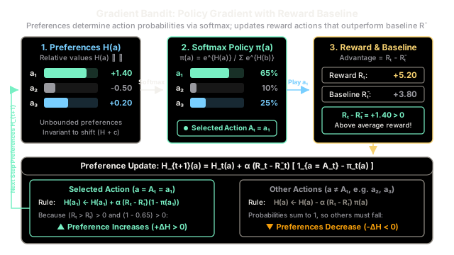
Why Does This Exist?

Most foundational multi-armed bandit algorithms—such as $\varepsilon$ -greedy, Upper Confidence Bound (UCB), and Thompson Sampling—are action-value methods. They maintain numerical estimates $Q(a)$ of the true expected payoff $q_*(a)$ for each arm, selecting actions based on which estimate is highest.

However, estimating absolute reward values introduces several practical and theoretical challenges:

Relative order matters, absolute magnitude does not: If arm 1 produces an expected return of $+102$ and arm 2 produces $+100$ , an agent does not need to estimate the number $102$ to understand that arm 1 is superior. Value estimators waste statistical effort calibrating arbitrary scales and offsets.
Rigid exploration policies: Action-value methods select actions through discontinuous operations (like $\arg\max$ ) combined with heuristic random exploration ( $\varepsilon$ ). They lack a natural, smooth mechanism to continuously adjust the probability of taking actions in proportion to evidence.
No direct path to policy optimization: In complex or continuous decision problems, estimating values everywhere is intractable. We need methods that directly parameterize and optimize the decision policy itself.

Gradient bandits resolve this by abandoning reward estimation altogether. Instead of tracking expected payouts, the agent assigns an unconstrained numerical preference $H_t(a) \in \mathbb{R}$ to each action. These preferences are converted into a probability distribution via a softmax transformation and optimized directly using stochastic gradient ascent on the expected total reward. Gradient bandits serve as the direct conceptual foundation for modern Policy Gradient Methods.

Think of It Like This

A radio DJ tuning genre weights against listener mood

Imagine a radio DJ deciding which genre of music—Pop, Rock, Hip-Hop, or Jazz—to broadcast next. Instead of trying to predict the exact number of phone calls or ratings each individual song will receive, the DJ maintains an internal "preference dial" for each genre.

Whenever it is time to queue a track, the DJ spins a roulette wheel where each genre's slice corresponds to its current preference dial (the softmax distribution). Higher dials get played more often, but every genre retains a chance to hit the airwaves.

After playing a song, the DJ checks listener feedback (the reward $R_t$ ) against the station's recent running average satisfaction score (the baseline $\bar{R}_t$ ):

Above-average reaction ( $R_t > \bar{R}_t$ ): A hip-hop track scores $8.5$ when the station average is $6.0$ . The DJ nudges the hip-hop dial upward. Because all probabilities must sum to $100\%$ , the other genres automatically surrender a fraction of their airtime.
Below-average reaction ( $R_t < \bar{R}_t$ ): An indie rock track scores $4.5$ . Even though the rating is positive and listeners did not boycott the station, it scored below the room average. The DJ dials down indie rock, causing the other genres to gain relative probability.

The DJ never needs to define what a "perfect 10" track feels like. They simply boost choices that beat the baseline and suppress choices that lag behind it.

Where the analogy stops: A human DJ must consider listener fatigue, time-of-day dynamics, and smooth transitions between songs. In a gradient bandit, trials are independent, arm payoff distributions are stationary, and there are no sequential state transitions.

How It Actually Works

Action Preferences and Stochastic Gradient Ascent

Rather than estimating expected payoffs $Q(a) \approx q_*(a)$ , a gradient bandit maintains a numerical preference $H_t(a) \in \mathbb{R}$ for each action $a \in \{1, 2, \dots, k\}$ .

Preferences have no units of reward. Only the relative differences between preferences dictate action selection. If you add an arbitrary constant $c$ to every preference, the action probabilities remain completely unchanged:

$\frac{e^{H_t(a) + c}}{\sum_{b=1}^k e^{H_t(b) + c}} = \frac{e^c \cdot e^{H_t(a)}}{e^c \sum_{b=1}^k e^{H_t(b)}} = \frac{e^{H_t(a)}}{\sum_{b=1}^k e^{H_t(b)}} = \pi_t(a)$

1. Softmax Action Selection

At time step $t$ , the probability of selecting action $a$ is determined by the softmax (Boltzmann / Gibbs) distribution:

$\pi_t(a) = \Pr(A_t = a) = \frac{e^{H_t(a)}}{\sum_{b=1}^k e^{H_t(b)}}$

Every action always has a strictly positive probability ( $\pi_t(a) > 0$ ), guaranteeing continuous exploration without requiring an artificial $\varepsilon$ -greedy exploration floor.

2. The Objective Function

The agent seeks to maximize expected reward across trials:

$\mathbb{E}[R_t] = \sum_{x=1}^k \pi_t(x) q_*(x)$

where $q_*(x) = \mathbb{E}[R_t \mid A_t = x]$ is the true underlying mean reward of action $x$ .

3. Deriving the Gradient

To perform gradient ascent, we take the derivative of expected reward with respect to preference $H_t(a)$ :

$\frac{\partial \mathbb{E}[R_t]}{\partial H_t(a)} = \sum_{x=1}^k q_*(x) \frac{\partial \pi_t(x)}{\partial H_t(a)}$

Using the derivative of the softmax function $\frac{\partial \pi_t(x)}{\partial H_t(a)} = \pi_t(x)(\mathbf{1}_{x=a} - \pi_t(a))$ , we can introduce an arbitrary baseline $B_t$ that does not depend on the action $x$ . Because probabilities sum to 1 ( $\sum_x \pi_t(x) = 1$ ), the gradient of the baseline term vanishes:

$\sum_{x=1}^k B_t \frac{\partial \pi_t(x)}{\partial H_t(a)} = B_t \frac{\partial}{\partial H_t(a)} \sum_{x=1}^k \pi_t(x) = B_t \frac{\partial (1)}{\partial H_t(a)} = 0$

Subtracting this zero-valued baseline yields:

$\frac{\partial \mathbb{E}[R_t]}{\partial H_t(a)} = \sum_{x=1}^k (q_*(x) - B_t) \pi_t(x) \left(\mathbf{1}_{x=a} - \pi_t(a)\right) = \mathbb{E}\left[ (R_t - \bar{R}_t) (\mathbf{1}_{A_t=a} - \pi_t(a)) \right]$

Replacing the true expectation with the sampled reward $R_t$ gives an unbiased stochastic gradient sample!

4. The Preference Update Rule

After taking action $A_t$ and observing reward $R_t$ , the preferences are updated via:

$H_{t+1}(a) = H_t(a) + \alpha (R_t - \bar{R}_t) \left(\mathbf{1}_{a=A_t} - \pi_t(a)\right) \quad \text{for all } a$

Breaking this into the chosen versus unchosen actions:

For the chosen arm ( $a = A_t$ ): $H_{t+1}(A_t) = H_t(A_t) + \alpha (R_t - \bar{R}_t)(1 - \pi_t(A_t))$
For all other arms ( $a \neq A_t$ ): $H_{t+1}(a) = H_t(a) - \alpha (R_t - \bar{R}_t)\pi_t(a)$

where:

$\alpha > 0$ is the step-size parameter (learning rate).
$\mathbf{1}_{a=A_t}$ is the indicator function ( $1$ if $a = A_t$ , else $0$ ).
$\bar{R}_t$ is the average reward baseline up to time $t$ , tracked incrementally:

$\bar{R}_t = \bar{R}_{t-1} + \frac{1}{t} (R_t - \bar{R}_{t-1}) \quad (\text{with } \bar{R}_1 = R_1)$

5. Role of the Average Reward Baseline

The baseline $\bar{R}_t$ acts as a comparative anchor. If an arm yields $R_t > \bar{R}_t$ , its preference climbs and all other preferences decline. If $R_t < \bar{R}_t$ , its preference falls even if $R_t > 0$ . While any baseline leaves the expected gradient mathematically unbiased, using the running average $\bar{R}_t$ dramatically reduces the variance of the gradient estimates, stabilizing learning.

Worked numerical example

Consider a 2-armed bandit ( $k = 2$ ) with step-size $\alpha = 0.20$ .

Initial State ( $t = 1$ )

Initial preferences: $H_1(a_1) = 0.00$ , $H_1(a_2) = 0.00$ .
Initial probabilities: $\pi_1(a_1) = \frac{e^0}{e^0 + e^0} = 0.5000, \quad \pi_1(a_2) = 0.5000$
Running baseline prior: $\bar{R}_1 = 4.00$ .

Round 1: Good Outcome on Arm 1

Action selected: The agent samples Arm $a_1$ ( $A_1 = a_1$ ).
Reward received: $R_1 = 6.00$ .
Advantage calculation: $R_1 - \bar{R}_1 = 6.00 - 4.00 = +2.00$ (performed above baseline).
Update chosen arm ( $a_1$ ): $H_2(a_1) = 0.00 + 0.20 \times (+2.00) \times (1 - 0.5000) = 0.00 + 0.2000 = +0.2000$
Update unchosen arm ( $a_2$ ): $H_2(a_2) = 0.00 - 0.20 \times (+2.00) \times 0.5000 = 0.00 - 0.2000 = -0.2000$
Update baseline: $\bar{R}_2 = 4.00 + \frac{1}{2}(6.00 - 4.00) = 5.00$
New probabilities for Round 2: $e^{H_2(a_1)} = e^{+0.20} \approx 1.2214, \quad e^{H_2(a_2)} = e^{-0.20} \approx 0.8187$ $\text{Sum} = 1.2214 + 0.8187 = 2.0401$ $\pi_2(a_1) = \frac{1.2214}{2.0401} \approx 0.5987 \; (59.87\%), \quad \pi_2(a_2) = \frac{0.8187}{2.0401} \approx 0.4013 \; (40.13\%)$

Arm $a_1$ 's probability jumped from $50.0\%$ to $59.9\%$ because it outperformed the average baseline.

Round 2: Poor Outcome on Arm 2

Action selected: The agent explores Arm $a_2$ ( $A_2 = a_2$ ).
Reward received: $R_2 = 2.00$ .
Advantage calculation: $R_2 - \bar{R}_2 = 2.00 - 5.00 = -3.00$ (performed below baseline).
Update chosen arm ( $a_2$ ): $H_3(a_2) = -0.2000 + 0.20 \times (-3.00) \times (1 - 0.4013) = -0.2000 - 0.60 \times 0.5987 = -0.2000 - 0.3592 = -0.5592$
Update unchosen arm ( $a_1$ ): $H_3(a_1) = +0.2000 - 0.20 \times (-3.00) \times 0.5987 = +0.2000 + 0.3592 = +0.5592$
New probabilities for Round 3: $e^{H_3(a_1)} = e^{+0.5592} \approx 1.7493, \quad e^{H_3(a_2)} = e^{-0.5592} \approx 0.5717$ $\text{Sum} = 1.7493 + 0.5717 = 2.3210$ $\pi_3(a_1) = \frac{1.7493}{2.3210} \approx 0.7537 \; (75.37\%), \quad \pi_3(a_2) = \frac{0.5717}{2.3210} \approx 0.2463 \; (24.63\%)$

Even though Arm $a_2$ delivered a positive reward of $+2.00$ , because it fell short of the $+5.00$ baseline, its preference plummeted and Arm $a_1$ 's selection probability climbed to $75.4\%$ .

Code

Below is a self-contained, type-hinted Python implementation of the Gradient Bandit algorithm with running baseline tracking.

1import math2import random3from typing import List4
5
6class GradientBandit:7    """Gradient Bandit algorithm with numerical preferences and baseline tracking.8
9    Optimizes numerical action preferences H(a) via stochastic gradient ascent10    on expected reward, parameterizing a softmax exploration policy.11    """12
13    def __init__(14        self,15        k_arms: int,16        alpha: float = 0.1,17        use_baseline: bool = True,18    ) -> None:19        self.k: int = k_arms20        self.alpha: float = alpha21        self.use_baseline: bool = use_baseline22        # Action preferences H_t(a), initialized to 0.023        self.preferences: List[float] = [0.0] * k_arms24        # Running average reward baseline R_bar25        self.baseline: float = 0.026        # Time step counter27        self.step_count: int = 028
29    def get_probabilities(self) -> List[float]:30        """Compute action probabilities using numerically stable softmax."""31        max_h = max(self.preferences)32        # Subtract max preference to prevent floating-point exponential overflow33        exp_h = [math.exp(h - max_h) for h in self.preferences]34        total_exp = sum(exp_h)35        return [e / total_exp for e in exp_h]36
37    def select_action(self) -> int:38        """Sample an action according to softmax probabilities pi_t."""39        probs = self.get_probabilities()40        r = random.random()41        cumulative = 0.042        for action_idx, p in enumerate(probs):43            cumulative += p44            if r < cumulative:45                return action_idx46        return self.k - 147
48    def update(self, action: int, reward: float) -> None:49        """Update action preferences and baseline following an observed reward."""50        self.step_count += 151        probs = self.get_probabilities()52
53        # Update average reward baseline incrementally if enabled54        if self.use_baseline:55            self.baseline += (reward - self.baseline) / self.step_count56            baseline_val = self.baseline57        else:58            baseline_val = 0.059
60        advantage = reward - baseline_val61
62        # Stochastic gradient update rule:63        # H_{t+1}(a) = H_t(a) + alpha * (R_t - R_bar) * (1_{a=A_t} - pi_t(a))64        for a in range(self.k):65            indicator = 1.0 if a == action else 0.066            self.preferences[a] += self.alpha * advantage * (indicator - probs[a])67
68
69# Example demonstration on a 3-armed bandit:70if __name__ == "__main__":71    random.seed(42)72
73    # 3-armed bandit environment with true payout means74    k = 375    true_means = [2.0, 5.0, 3.0]  # Arm index 1 is optimal76    agent = GradientBandit(k_arms=k, alpha=0.2, use_baseline=True)77
78    print("Initial preferences:", [round(h, 3) for h in agent.preferences])79    print("Initial probabilities:", [round(p, 3) for p in agent.get_probabilities()])80
81    # Train for 500 interaction rounds82    for _ in range(500):83        a = agent.select_action()84        # Sample reward with Gaussian noise around true arm mean85        r = random.gauss(true_means[a], 1.0)86        agent.update(action=a, reward=r)87
88    probs = agent.get_probabilities()89    print("Final preferences:", [round(h, 3) for h in agent.preferences])90    print("Final probabilities:", [round(p, 3) for p in probs])91    print(f"Optimal arm (index 1) probability: {probs[1]:.1%}")92    print(f"Average baseline reward: {agent.baseline:.2f}")93
94# -> Expected output:95# Initial preferences: [0.0, 0.0, 0.0]96# Initial probabilities: [0.333, 0.333, 0.333]97# Final preferences: [-2.359, 4.792, -2.433]98# Final probabilities: [0.001, 0.998, 0.001]99# Optimal arm (index 1) probability: 99.8%100# Average baseline reward: 4.90

Watch Out For

Omitting the reward baseline in positive-reward environments

A common mistake when implementing gradient bandits is omitting the reward baseline ( $\bar{R}_t = 0$ ), assuming that stochastic gradient ascent will still converge because the baseline term has an expected gradient of zero.

The failure mode: If all observed rewards are strictly positive (for example, payouts centered around $+100$ ), every single action pull produces $R_t - 0 > 0$ . As a consequence:

Every time any arm is pulled, its preference $H_t(a)$ is bumped upward.
Even severely suboptimal arms receive continuous positive reinforcement simply by being explored.
Preferences of all actions grow large and positive simultaneously. Suboptimal arms only experience relative decreases through the normalizer $\sum_b e^{H(b)}$ , but their probabilities decline at an agonizingly slow rate.

The symptom: The agent exhibits massive gradient variance, takes thousands of extra steps to converge, or prematurely locks onto the first arm tested simply because early rewards boosted its preference ahead of the pack.

The fix: Always maintain a running average reward baseline $\bar{R}_t = \bar{R}_{t-1} + \frac{1}{t}(R_t - \bar{R}_{t-1})$ . The baseline centers the reward signals around zero, ensuring that below-average rewards actively depress preferences ( $R_t - \bar{R}_t < 0$ ) and quickly reallocate exploration budget to promising arms.

The Quick Version

Preferences, not values: Gradient bandits maintain unbounded numerical preferences $H_t(a) \in \mathbb{R}$ rather than estimating expected reward values $Q(a)$ .
Softmax exploration: Action selection probabilities $\pi_t(a) \propto e^{H_t(a)}$ naturally balance exploration without requiring hard cutoff thresholds or artificial $\varepsilon$ -greedy coin flips.
Relative performance drives updates: The update rule $H_{t+1}(a) = H_t(a) + \alpha (R_t - \bar{R}_t)(\mathbf{1}_{a=A_t} - \pi_t(a))$ rewards actions that beat the running average baseline $\bar{R}_t$ and penalizes actions that fall below it.
The baseline is vital: While theoretically unbiased without a baseline, omitting $\bar{R}_t$ causes preferences to drift upward unboundedly when rewards are positive, resulting in severe variance and crippled convergence.
Foundation of policy gradients: Gradient bandits are the single-state formulation of the Policy Gradient Theorem, directly inspiring algorithms like REINFORCE and PPO.