Maximum Entropy Inverse Reinforcement Learning

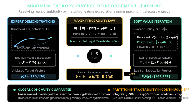
Maximum Entropy Inverse Reinforcement Learning infers hidden reward functions from expert demonstrations without making unjustified preferences between equally good trajectories. By framing trajectory probability as an exponential energy model, it resolves the fundamental ambiguity of ill-posed inverse problems through the principle of maximum entropy.

Why Does This Exist?

In classical reinforcement learning, an engineer specifies a scalar reward function, and the agent optimizes a policy to maximize cumulative return. In many real-world domains—such as autonomous highway navigation, robotic surgery, and human-assistive devices—handcrafting an explicit scalar reward function is notoriously brittle. A tiny misspecification leads to reward hacking, where the agent maximizes the literal score while exhibiting dangerous behavior.

Inverse Reinforcement Learning (IRL) inverts the paradigm: given demonstrations executed by an expert, IRL infers the underlying reward function that explains the observed behavior. However, classical IRL formulations face a fundamental mathematical bottleneck known as reward ambiguity. As demonstrated by Ng and Russell (2000), infinitely many reward functions explain any given demonstration policy. The degenerate reward function $R(s) = 0$ for all states trivially makes every conceivable trajectory optimal. Furthermore, max-margin apprenticeship methods (Abbeel and Ng, 2004) resolve ties between multiple trajectories arbitrarily, assuming an unnaturally rigid expert who never makes sub-optimal mistakes or explores alternative routes with equal return.

Maximum Entropy Inverse Reinforcement Learning (MaxEnt IRL), formulated by Brian Ziebart et al. (2008), resolves this ill-posed ambiguity using E.T. Jaynes' Principle of Maximum Entropy. Instead of assuming deterministic optimality, MaxEnt IRL models the probability of any trajectory as an exponential function of its total reward. Among all trajectory distributions that match the expert's expected feature counts, MaxEnt IRL chooses the unique distribution that maximizes Shannon information entropy. This mathematical framing guarantees that the learner commits to zero unjustified preferences between equally rewarding trajectories, naturally absorbs stochastic human demonstration noise, and establishes an exact, globally concave optimization objective.

Think of It Like This

Inferring a Master Chef's Secret Sauce Recipe

Imagine you are a food scientist trying to reverse-engineer a three-star Michelin chef's secret vinaigrette recipe by observing 50 line cooks who were trained under the chef. Every bottle prepared by a line cook tastes balanced, but no two bottles contain the exact same microscopic milliliters of olive oil, lemon juice, Dijon mustard, and sea salt.

If you modeled the cooks with rigid, deterministic rules, any slight difference between two bottles would appear completely contradictory: you would fail to infer a recipe because the demonstrations do not follow an identical single path. Conversely, if you used a naive reward threshold where any recipe that doesn't spoil is acceptable, a plain cup of tap water would trivially pass as "valid."

MaxEnt IRL acts like a thermodynamic flavor analyst. It assumes that the chef's kitchen follows a Boltzmann energy distribution: recipes with higher culinary balance have exponentially higher odds of being prepared, but random line-cook variation produces natural thermal noise around that optimum.

Most importantly, when you compute the average acidity and oiliness across all 50 sample bottles, thousands of potential spice combinations could produce that exact average. The Maximum Entropy principle demands that you choose the recipe distribution with the highest possible variety (maximum entropy)—refusing to introduce imaginary secret ingredients (like truffle oil or cardamom) that are not strictly demanded by the empirical flavor data.

Where the analogy stops: Culinary ingredients are blended simultaneously in a single mixing bowl, whereas an MDP expert executes sequential, state-dependent decisions over time, where early turns alter the reachable state space of all subsequent decisions.

How It Actually Works

The Maximum Entropy Trajectory Formulation and Soft Dynamic Programming

Consider a Markov Decision Process (MDP) defined by states $\mathcal{S}$ , actions $\mathcal{A}$ , transition probabilities $P(s' \mid s, a)$ , discount factor $\gamma \in (0, 1]$ , and a feature vector $\phi(s) \in \mathbb{R}^k$ mapping each state to $k$ measurable features.

The true reward function is parameterized as a linear combination of state features with an unknown weight vector $\theta \in \mathbb{R}^k$ :

R_\theta(s) = \theta^T \phi(s)

A demonstration trajectory $\tau$ of horizon $T$ consists of a sequence of states and actions: $\tau = (s_0, a_0, s_1, a_1, \dots, s_T)$ . The total feature count of trajectory $\tau$ is the sum of features encountered along its path:

\mu_\tau = \sum_{t=0}^T \phi(s_t)

The total return of trajectory $\tau$ under weights $\theta$ is:

R_\theta(\tau) = \sum_{t=0}^T R_\theta(s_t) = \theta^T \mu_\tau

Given a dataset of $N$ expert demonstrations $\mathcal{D}_E = \{\tau_1, \tau_2, \dots, \tau_N\}$ , the empirical expert feature count vector is:

\tilde{\mu}_E = \frac{1}{N} \sum_{i=1}^N \mu_{\tau_i} = \frac{1}{N} \sum_{i=1}^N \sum_{t=0}^T \phi(s_{i, t})

1. The Maximum Entropy Principle

MaxEnt IRL seeks a trajectory probability distribution $P(\tau)$ that maximizes trajectory Shannon entropy $H(P) = -\sum_\tau P(\tau) \log P(\tau)$ , subject to the constraint that the learner's expected feature counts match the expert's empirical feature counts:

\max_{P} -\sum_{\tau} P(\tau) \log P(\tau) \quad \text{subject to} \quad \sum_{\tau} P(\tau) \mu_\tau = \tilde{\mu}_E, \quad \sum_{\tau} P(\tau) = 1

Using Lagrange multipliers, the unique distribution solving this constrained optimization problem is the Boltzmann (exponential energy) distribution:

P(\tau \mid \theta) = \frac{1}{Z(\theta)} \exp(R_\theta(\tau)) = \frac{1}{Z(\theta)} \exp(\theta^T \mu_\tau)

where $Z(\theta)$ is the partition function normalizing the distribution across all conceivable trajectories:

Z(\theta) = \sum_{\tau} \exp(\theta^T \mu_\tau)

2. The Log-Likelihood Objective and Gradient

Under this exponential distribution, the log-likelihood of the expert dataset $\mathcal{D}_E$ under parameters $\theta$ is:

\mathcal{L}(\theta) = \frac{1}{N} \sum_{\tau \in \mathcal{D}_E} \log P(\tau \mid \theta) = \theta^T \tilde{\mu}_E - \log Z(\theta)

Taking the analytical gradient of $\mathcal{L}(\theta)$ with respect to the reward parameter vector $\theta$ :

\nabla_\theta \mathcal{L}(\theta) = \tilde{\mu}_E - \frac{1}{Z(\theta)} \sum_{\tau} \mu_\tau \exp(\theta^T \mu_\tau) = \tilde{\mu}_E - \mathbb{E}_{P(\tau \mid \theta)}[\mu]

This gradient has an intuitive form: the difference between empirical expert feature expectations and learner expected feature counts.

Because $\mathcal{L}(\theta)$ is strictly concave with respect to linear weights $\theta$ , gradient ascent is guaranteed to converge to the global maximum likelihood solution with zero local minima:

\theta \leftarrow \theta + \alpha \cdot \left(\tilde{\mu}_E - \mathbb{E}_{P(\tau \mid \theta)}[\mu]\right)

3. Efficient Computation via Soft Dynamic Programming

Summing over all possible trajectories to evaluate $Z(\theta)$ and $\mathbb{E}[\mu]$ directly is intractable in multi-step MDPs because the number of trajectories grows exponentially with horizon $T$ . Ziebart et al. resolved this using a forward-backward soft dynamic programming algorithm:

Backward Pass (Soft Value Iteration): Compute soft action values and partition values backward from $t = T$ to $0$ :
$Q(s, a) = R_\theta(s) + \sum_{s'} P(s' \mid s, a) V(s')$ $V(s) = \operatorname{softmax}_a Q(s, a) = \log \sum_{a \in \mathcal{A}} \exp(Q(s, a))$ $\pi(a \mid s) = \exp(Q(s, a) - V(s)) = \frac{\exp(Q(s, a))}{\sum_{a'} \exp(Q(s, a'))}$
Forward Pass (State Visitation Frequency): Propagate expected state visitation frequencies forward in time:
$D_0(s) = P(s_0 = s)$ $D_{t+1}(s') = \sum_{s \in \mathcal{S}} \sum_{a \in \mathcal{A}} D_t(s) \pi(a \mid s) P(s' \mid s, a)$ $D(s) = \sum_{t=0}^T D_t(s)$
Feature Expectation Matching: Compute expected learner features as the inner product of state visitation frequencies and feature vectors:
$\mathbb{E}_{P(\tau \mid \theta)}[\mu] = \sum_{s \in \mathcal{S}} D(s) \phi(s)$

Worked numerical example

Let us trace a concrete, step-by-step numerical update for a 3-state navigation graph with a 2-dimensional feature representation.

Setup

Consider three states $s_1$ , $s_2$ , and $s_3$ (an absorbing goal):

$\phi(s_1) = [1.0, 0.0]$ (e.g., highway path feature)
$\phi(s_2) = [0.0, 1.0]$ (e.g., scenic side-road feature)
$\phi(s_3) = [1.0, 1.0]$ (terminal destination containing both attributes)

Two candidate trajectories reach $s_3$ :

Trajectory 1 ( $\tau_1$ ): Travels via $s_1 \to s_3$ . Feature count: $\mu_{\tau_1} = \phi(s_1) + \phi(s_3) = [1.0, 0.0] + [1.0, 1.0] = [2.0, 1.0]$
Trajectory 2 ( $\tau_2$ ): Travels via $s_2 \to s_3$ . Feature count: $\mu_{\tau_2} = \phi(s_2) + \phi(s_3) = [0.0, 1.0] + [1.0, 1.0] = [1.0, 2.0]$

Initial reward weight vector:

\theta = [1.0, 0.5]

Expert demonstration dataset: 10 total demonstrations, with 8 demonstrations choosing $\tau_1$ (80%) and 2 choosing $\tau_2$ (20%).

Step 1: Compute Trajectory Returns

Calculate $R_\theta(\tau) = \theta^T \mu_\tau$ :

For $\tau_1$ : $R_\theta(\tau_1) = (1.0 \times 2.0) + (0.5 \times 1.0) = 2.0 + 0.5 = 2.5000$
For $\tau_2$ : $R_\theta(\tau_2) = (1.0 \times 1.0) + (0.5 \times 2.0) = 1.0 + 1.0 = 2.0000$

Step 2: Compute the Partition Function $Z(\theta)$

Evaluate the unnormalized trajectory energies:

\exp(R_\theta(\tau_1)) = \exp(2.5) \approx 12.1825

\exp(R_\theta(\tau_2)) = \exp(2.0) \approx 7.3891

Sum across candidate trajectories to obtain the partition function:

Z(\theta) = 12.1825 + 7.3891 = 19.5716

Step 3: Compute Model Trajectory Probabilities

Determine the Boltzmann probabilities assigned to each path under current $\theta$ :

P(\tau_1 \mid \theta) = \frac{\exp(R_\theta(\tau_1))}{Z(\theta)} = \frac{12.1825}{19.5716} \approx 0.6225

P(\tau_2 \mid \theta) = \frac{\exp(R_\theta(\tau_2))}{Z(\theta)} = \frac{7.3891}{19.5716} \approx 0.3775

Notice that the current model assigns 62.25% probability to $\tau_1$ and 37.75% to $\tau_2$ .

Step 4: Compare Expert vs. Learner Feature Counts

Expert empirical feature counts $\tilde{\mu}_E$ :
$\tilde{\mu}_E = 0.80 \times \mu_{\tau_1} + 0.20 \times \mu_{\tau_2}$ $\tilde{\mu}_E = 0.80 \times [2.0, 1.0] + 0.20 \times [1.0, 2.0] = [1.60 + 0.20, 0.80 + 0.40] = [1.8000, 1.2000]$
Learner expected feature counts $\mathbb{E}_{P(\tau \mid \theta)}[\mu]$ :
$\mathbb{E}[\mu] = 0.6225 \times [2.0, 1.0] + 0.3775 \times [1.0, 2.0]$ $\mathbb{E}[\mu] = [1.2450 + 0.3775, 0.6225 + 0.7550] = [1.6225, 1.3775]$

Step 5: Compute Log-Likelihood Gradient and Parameter Update

Compute the gradient $\nabla_\theta \mathcal{L}(\theta) = \tilde{\mu}_E - \mathbb{E}[\mu]$ :

For feature 1: $\nabla_{\theta_1} \mathcal{L} = 1.8000 - 1.6225 = +0.1775$
For feature 2: $\nabla_{\theta_2} \mathcal{L} = 1.2000 - 1.3775 = -0.1775$

Gradient vector:

\nabla_\theta \mathcal{L}(\theta) = [+0.1775, -0.1775]

Apply a gradient ascent step with learning rate $\alpha = 1.0$ :

\theta_{\text{new}} = \theta + \alpha \cdot \nabla_\theta \mathcal{L}(\theta)

\theta_{\text{new}} = [1.0, 0.5] + 1.0 \times [+0.1775, -0.1775] = [1.1775, 0.3225]

Because the expert exhibits a stronger preference for feature 1 ( $1.80 > 1.6225$ ) than the current model predicts, the gradient update automatically boosts $\theta_1$ by $+0.1775$ while simultaneously discounting $\theta_2$ by $-0.1775$ . Over successive iterations, $\theta$ converges until the learner's expected feature counts match the expert counts within numerical precision.

Code

The following self-contained Python script implements the Maximum Entropy Inverse Reinforcement Learning objective, evaluates partition functions and Boltzmann trajectory probabilities using numerically stable Log-Sum-Exp operations, computes empirical feature gradients, and validates the numerical example step-by-step.

1from typing import Dict, List, Tuple2import numpy as np3
4class MaxEntIRL:5    """Maximum Entropy Inverse Reinforcement Learning (Ziebart et al., 2008).6
7    Infers reward weight vector theta by matching expert feature expectations8    under the maximum entropy trajectory distribution P(tau | theta) prop to exp(theta^T mu_tau).9    """10
11    def __init__(self, feature_dim: int, learning_rate: float = 1.0) -> None:12        self.feature_dim = feature_dim13        self.lr = learning_rate14        self.theta = np.zeros(feature_dim, dtype=np.float64)15
16    def compute_trajectory_probabilities(17        self,18        candidate_trajectories: List[np.ndarray],19        theta: np.ndarray,20    ) -> Tuple[np.ndarray, float]:21        """Computes Boltzmann probabilities P(tau | theta) and partition function Z."""22        # Trajectory returns R(tau) = theta^T mu_tau23        returns = np.array([float(np.dot(theta, mu)) for mu in candidate_trajectories])24
25        # Numerically stable Log-Sum-Exp computation: log Z = max_R + log sum exp(R - max_R)26        max_r = np.max(returns)27        log_z = max_r + np.log(np.sum(np.exp(returns - max_r)))28        z = float(np.exp(log_z))29
30        # Normalized trajectory probabilities31        probs = np.exp(returns - log_z)32        return probs, z33
34    def compute_expected_features(35        self,36        candidate_trajectories: List[np.ndarray],37        probs: np.ndarray,38    ) -> np.ndarray:39        """Computes expected learner feature counts E[mu] = sum_tau P(tau) mu_tau."""40        stacked_features = np.array(candidate_trajectories)41        return np.sum(probs[:, None] * stacked_features, axis=0)42
43    def compute_gradient(44        self,45        expert_feature_counts: np.ndarray,46        candidate_trajectories: List[np.ndarray],47        theta: np.ndarray,48    ) -> Tuple[np.ndarray, np.ndarray, float]:49        """Computes gradient of trajectory log-likelihood: grad L = mu_E - E_learner[mu]."""50        probs, z = self.compute_trajectory_probabilities(candidate_trajectories, theta)51        learner_features = self.compute_expected_features(candidate_trajectories, probs)52        gradient = expert_feature_counts - learner_features53        return gradient, learner_features, z54
55    def update_step(56        self,57        expert_feature_counts: np.ndarray,58        candidate_trajectories: List[np.ndarray],59    ) -> Dict[str, np.ndarray | float]:60        """Performs a single gradient ascent step to maximize trajectory likelihood."""61        gradient, learner_features, z = self.compute_gradient(62            expert_feature_counts, candidate_trajectories, self.theta63        )64        self.theta += self.lr * gradient65        return {66            "gradient": gradient,67            "learner_features": learner_features,68            "partition_function": z,69            "updated_theta": self.theta.copy(),70        }71
72# --- Verification Matching Worked Numerical Example ---73# State feature configurations: phi(s1)=[1, 0], phi(s2)=[0, 1], phi(s3)=[1, 1]74# Trajectory 1: s1 -> s3 => mu_tau1 = [2.0, 1.0]75# Trajectory 2: s2 -> s3 => mu_tau2 = [1.0, 2.0]76mu_tau1 = np.array([2.0, 1.0])77mu_tau2 = np.array([1.0, 2.0])78trajectories = [mu_tau1, mu_tau2]79
80# Expert dataset: 8 demonstrations of tau1, 2 of tau2 (80% / 20%)81mu_expert = 0.80 * mu_tau1 + 0.20 * mu_tau2  # [1.80, 1.20]82
83# Initial weights from worked example: theta = [1.0, 0.5]84irl = MaxEntIRL(feature_dim=2, learning_rate=1.0)85irl.theta = np.array([1.0, 0.5])86
87# Compute probabilities under initial theta88probs, z = irl.compute_trajectory_probabilities(trajectories, irl.theta)89step_info = irl.update_step(mu_expert, trajectories)90
91print(f"Partition function Z: {z:.4f}")92# -> Partition function Z: 19.571693
94print(f"Trajectory Probabilities: P(tau1)={probs[0]:.4f}, P(tau2)={probs[1]:.4f}")95# -> Trajectory Probabilities: P(tau1)=0.6225, P(tau2)=0.377596
97print(f"Expert Feature Counts: [{mu_expert[0]:.2f}, {mu_expert[1]:.2f}]")98# -> Expert Feature Counts: [1.80, 1.20]99
100learner_mu = step_info["learner_features"]101print(f"Learner Feature Counts: [{learner_mu[0]:.4f}, {learner_mu[1]:.4f}]")102# -> Learner Feature Counts: [1.6225, 1.3775]103
104grad = step_info["gradient"]105print(f"Likelihood Gradient: [{grad[0]:+.4f}, {grad[1]:+.4f}]")106# -> Likelihood Gradient: [+0.1775, -0.1775]107
108updated_w = step_info["updated_theta"]109print(f"Updated Parameters Theta: [{updated_w[0]:.4f}, {updated_w[1]:.4f}]")110# -> Updated Parameters Theta: [1.1775, 0.3225]111
112# Assertions matching worked example113np.testing.assert_allclose(z, 19.5716, atol=1e-3)114np.testing.assert_allclose(probs, [0.6225, 0.3775], atol=1e-4)115np.testing.assert_allclose(mu_expert, [1.80, 1.20], atol=1e-4)116np.testing.assert_allclose(learner_mu, [1.6225, 1.3775], atol=1e-4)117np.testing.assert_allclose(grad, [+0.1775, -0.1775], atol=1e-4)118np.testing.assert_allclose(updated_w, [1.1775, 0.3225], atol=1e-4)119print("MaxEnt IRL verification assertions passed successfully.")120# -> MaxEnt IRL verification assertions passed successfully.

Watch Out For

The Continuous Partition Function Explosion: Scaling Beyond Discrete State Graphs

In discrete, tabular MDPs with low horizons, the partition function $Z(\theta)$ can be computed exactly using soft backward-forward dynamic programming. However, when practitioners transition to high-dimensional continuous control problems (e.g., 7-DOF robotic arms or continuous autonomous driving), the partition function becomes an integral over an uncountably infinite set of continuous paths:

Z(\theta) = \int_{\tau} \exp\left(R_\theta(\tau)\right) d\tau

Symptom: Attempting to discretize continuous state spaces causes an exponential memory explosion ( $O(K^d)$ where $d$ is dimension). If practitioners attempt naive Monte Carlo sampling to estimate $Z(\theta)$ , the sample variance diverges catastrophically because high-reward trajectories occupy an infinitesimally tiny fraction of the total continuous trajectory volume.

Concrete Fix:

Guided Cost Learning (GCL): Use an adaptive importance sampling distribution $q(\tau)$ that trains alongside the reward function, focusing samples in high-reward trajectory corridors: $Z(\theta) \approx \frac{1}{M} \sum_{j=1}^M \frac{\exp(R_\theta(\tau_j))}{q(\tau_j)}, \quad \tau_j \sim q(\tau)$
Generative Adversarial Imitation Learning (GAIL): Replace explicit partition function calculation entirely. By defining an adversarial game between a generator policy $\pi_\theta$ and a discriminator $D_\psi(s, a)$ , GAIL minimizes the Jensen-Shannon divergence between expert and learner state-action distributions, recovering the MaxEnt policy directly without ever evaluating $Z(\theta)$ .

The Quick Version

Solves Reward Ambiguity: In classical IRL, infinitely many reward functions explain expert demonstrations (including trivial $R(s) = 0$ ). MaxEnt IRL resolves this by selecting the unique trajectory distribution that maximizes Shannon entropy while matching expert feature counts.
Unbiased Trajectory Distribution: By modeling trajectory probabilities with an exponential Gibbs distribution $P(\tau) \propto \exp(R(\tau))$ , it treats trajectories with equal return with equal probability, eliminating arbitrary algorithmic bias.
Globally Concave Optimization: When reward functions are linear in state features, the trajectory log-likelihood objective is strictly concave, guaranteeing that standard gradient ascent finds the globally optimal reward weights without local optima.
Elegant Gradient Rule: The gradient with respect to reward parameters is simply the difference between empirical expert feature expectations and expected learner feature counts: $\nabla_\theta \mathcal{L} = \tilde{\mu}_E - \mathbb{E}_{P}[\mu]$ .