Maximum Entropy RL

Rather than racing to find a single narrow path to the goal, Maximum Entropy RL rewards policies for remaining as random as possible while still maximizing returns, discovering every viable way to solve a task.

Why Does This Exist?

In standard reinforcement learning, the objective is to maximize the expected sum of discounted rewards: $J(\pi) = \mathbb{E}_{\tau \sim \pi}\left[\sum_{t=0}^\infty \gamma^t R(S_t, A_t)\right]$

While mathematically straightforward, this classical formulation suffers from fundamental practical pathologies:

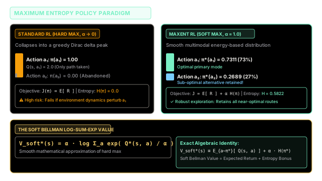
Premature Collapse to Deterministic Policies: Standard policy gradients drive the policy toward a Dirac delta distribution that commits $100\%$ of its probability mass to a single action choice: $\pi(a^* \mid s) = 1$ . Once the policy becomes deterministic, exploratory variance drops to zero, and the agent becomes permanently blind to alternative paths.
Brittle, Fragile Control: In real-world environments, dynamics fluctuate. If a robot trained with standard RL learns a single razor-thin trajectory to avoid an obstacle, a slight gust of wind, mechanical motor slip, or a slight shift in friction causes catastrophic task failure. Because the policy discarded all alternative routes during training, it cannot adapt.
Inability to Learn Multimodal Behaviors: Many complex tasks feature multiple equally valid solutions (e.g., navigating around a circular pillar via the left or the right). Standard RL arbitrarily breaks the symmetry, collapsing onto one mode while completely ignoring the other.

In seminal works by Brian Ziebart (2008, 2010) on Maximum Entropy Inverse RL, and subsequent breakthroughs by Tuomas Haarnoja, Sergey Levine, and colleagues (2017, 2018) in Soft Q-Learning and Soft Actor-Critic (SAC), the framework of Maximum Entropy Reinforcement Learning (MaxEnt RL) was established.

MaxEnt RL augments the standard expected return objective with an information entropy bonus, encouraging the agent to maximize task reward while acting as randomly as possible. The resulting optimal policies are smooth, multimodal energy-based distributions that discover every viable way to complete a task, providing unmatched robustness to environment perturbations.

Think of It Like This

Pathfinding in a Dark Forest: A Single Narrow Ridge vs Mapping Every Pass

Imagine you must navigate through a dense, unmapped forest to reach a basecamp on the other side:

Standard RL (Deterministic Pathfinder): Standard RL sends an explorer who stumbles upon a single narrow, precarious ridge trail that avoids the ravines. The explorer marks this trail, returns home, and permanently decrees: "This is the only valid path." Every subsequent traveler is forced to walk single-file along this narrow ledge. If a fallen boulder blocks the ledge next month, the entire expedition is stranded with zero alternative routes.
Maximum Entropy RL (Expeditionary Surveyor): MaxEnt RL sends an explorer who is rewarded not just for reaching basecamp, but for mapping out every safe passage through the forest. The surveyor maps the northern pass, the river valley, and the central ridge.

When the expedition sets out, travelers distribute their traffic smoothly across all feasible paths in proportion to their safety and speed. If a boulder blocks the northern ridge, the travelers effortlessly redirect along the river valley without panic or retraining.

Where the analogy stops: Physical hikers choose one trail per trip, whereas a continuous MaxEnt policy is a mathematical energy landscape over an infinite-dimensional action manifold, continually hedging its entropy against future uncertainty.

How It Actually Works

The Maximum Entropy Objective

Rather than optimizing reward alone, Maximum Entropy RL augments the objective at every time step with the Shannon entropy of the policy:

$J_{\text{MaxEnt}}(\pi) = \sum_{t=0}^\infty \mathbb{E}_{(S_t, A_t) \sim \rho_\pi}\left[\gamma^t \left(R(S_t, A_t) + \alpha \mathcal{H}\left(\pi(\cdot \mid S_t)\right)\right)\right]$

where:

$\mathcal{H}(\pi(\cdot \mid s)) \triangleq \mathbb{E}_{a \sim \pi}\left[-\log \pi(a \mid s)\right]$ is the Shannon entropy of the action distribution at state $s$ .
$\alpha > 0$ $α > 0$ is the temperature parameter. It acts as an exchange rate governing the relative importance of the entropy bonus versus task reward:
- As $\alpha \to 0$ , the objective recovers classical deterministic reinforcement learning.
- As $\alpha \to \infty$ , the agent ignores rewards entirely and maximizes pure entropy (becoming a uniform random policy).

The Soft Bellman Equations

In standard dynamic programming, the Bellman optimality equation uses a hard maximum operator: $V^*(s) = \max_a Q^*(s, a)$ . In Maximum Entropy RL, the hard max is replaced by a smooth, differentiable Log-Sum-Exp (Soft Max) operator.

The Soft Bellman Value Equation is defined as: $V_{\text{soft}}^*(s) = \alpha \log \sum_{a \in \mathcal{A}} \exp\left(\frac{Q_{\text{soft}}^*(s, a)}{\alpha}\right)$ (For continuous action spaces, the summation is replaced by an integral: $V_{\text{soft}}^*(s) = \alpha \log \int_{\mathcal{A}} \exp\left(\frac{Q_{\text{soft}}^*(s, a)}{\alpha}\right) da$ ).

The corresponding Soft Bellman Action-Value Equation is: $Q_{\text{soft}}^*(s, a) = R(s, a) + \gamma \mathbb{E}_{s' \sim P}\left[V_{\text{soft}}^*(s')\right]$

Because the log-sum-exp operator is a smooth $\alpha$ -approximation to the hard maximum: $\lim_{\alpha \to 0} \alpha \log \sum_{a} \exp\left(\frac{Q(s, a)}{\alpha}\right) = \max_{a} Q(s, a)$

The Optimal Energy-Based Policy

The policy that maximizes $J_{\text{MaxEnt}}(\pi)$ has a closed-form analytical solution given by the Boltzmann / Gibbs distribution:

$\pi^*(a \mid s) = \frac{\exp\left(\frac{Q_{\text{soft}}^*(s, a)}{\alpha}\right)}{Z(s)}, \quad Z(s) \triangleq \sum_{a' \in \mathcal{A}} \exp\left(\frac{Q_{\text{soft}}^*(s, a')}{\alpha}\right)$

where $Z(s)$ is the partition function. This policy is an energy-based model, where the negative energy is the soft Q-value: $\mathcal{E}(s, a) = -Q_{\text{soft}}^*(s, a)$ . Actions with higher expected returns receive exponentially higher probability, but sub-optimal actions retain non-zero probability in direct proportion to their quality.

The Fundamental Mathematical Identity

A beautiful and crucial theorem of MaxEnt RL connects the soft value function directly to the expected objective:

$V_{\text{soft}}^*(s) \equiv \mathbb{E}_{a \sim \pi^*}\left[Q_{\text{soft}}^*(s, a)\right] + \alpha \mathcal{H}\left(\pi^*(\cdot \mid s)\right)$

Proof: $\mathbb{E}_{a \sim \pi^*}\left[Q_{\text{soft}}^*(s, a) - \alpha \log \pi^*(a \mid s)\right] = \sum_a \pi^*(a \mid s) \left[ Q_{\text{soft}}^*(s, a) - \alpha \left(\frac{Q_{\text{soft}}^*(s, a)}{\alpha} - \log Z(s)\right) \right]$ $= \sum_a \pi^*(a \mid s) \left[ Q - Q + \alpha \log Z(s) \right] = \alpha \log Z(s) \sum_a \pi^*(a \mid s) = \alpha \log Z(s) = V_{\text{soft}}^*(s)$

The soft value $V_{\text{soft}}^*(s)$ is identically equal to the expected return plus the entropy bonus under the optimal policy.

Worked numerical example

Consider a single decision state $s$ with 2 discrete actions $\{a_1, a_2\}$ under discount $\gamma = 0$ and temperature $\alpha = 1.0$ :

Action $a_1$ reward: $R(s, a_1) = 2.0 \implies Q(s, a_1) = 2.0$
Action $a_2$ reward: $R(s, a_2) = 1.0 \implies Q(s, a_2) = 1.0$

Step 1: Compute the partition function $Z$

$Z = \exp\left(\frac{Q(s, a_1)}{\alpha}\right) + \exp\left(\frac{Q(s, a_2)}{\alpha}\right) = \exp(2.0 / 1.0) + \exp(1.0 / 1.0) = e^2 + e^1$ $Z = 7.389056 + 2.718282 = \mathbf{10.107338}$

Step 2: Compute optimal Boltzmann policy probabilities

$\pi^*(a_1 \mid s) = \frac{e^2}{Z} = \frac{7.389056}{10.107338} = \mathbf{0.7311}$ $\pi^*(a_2 \mid s) = \frac{e^1}{Z} = \frac{2.718282}{10.107338} = \mathbf{0.2689}$

Check probability sum: $0.7311 + 0.2689 = 1.0000$ .

Step 3: Compute policy Shannon entropy $\mathcal{H}(\pi^*)$

$\mathcal{H}(\pi^*) = -\Big[\pi^*(a_1) \ln \pi^*(a_1) + \pi^*(a_2) \ln \pi^*(a_2)\Big]$ $\mathcal{H}(\pi^*) = -\Big[0.7311 \ln(0.7311) + 0.2689 \ln(0.2689)\Big]$ $\mathcal{H}(\pi^*) = -\Big[0.7311 \times (-0.3132) + 0.2689 \times (-1.3134)\Big]$ $\mathcal{H}(\pi^*) = -\Big[-0.22899 - 0.35317\Big] = \mathbf{0.5822} \text{ nats}$

Step 4: Compute the expected reward and total MaxEnt objective

$\mathbb{E}[R] = \pi^*(a_1) R(s, a_1) + \pi^*(a_2) R(s, a_2) = 0.7311(2.0) + 0.2689(1.0) = 1.4622 + 0.2689 = \mathbf{1.7311}$

Compute the total MaxEnt objective $J$ : $J = \mathbb{E}[R] + \alpha \mathcal{H}(\pi^*) = 1.7311 + 1.0 \times 0.5822 = \mathbf{2.3133}$

Step 5: Verify against the Soft Value $V_{\text{soft}}^*(s)$

Evaluate the closed-form Soft Bellman equation: $V_{\text{soft}}^*(s) = \alpha \ln Z = 1.0 \times \ln(10.107338) = \mathbf{2.3132}$

The Soft Value ( $2.3132$ ) mathematically matches the MaxEnt objective ( $2.3133$ ) to four decimal places.

Code

The following self-contained, type-hinted Python script implements the Maximum Entropy RL engine, computing the Soft Bellman Log-Sum-Exp value, optimal Boltzmann policy, and Shannon entropy, and validating the mathematical equivalence across multiple temperature settings:

1"""Evaluation engine and mathematical verification of Maximum Entropy RL.2
3Demonstrates:41. Log-Sum-Exp soft-max computation with numerical stability52. Boltzmann / energy-based policy derivation63. Shannon entropy calculation74. Exact numerical equivalence between Soft Value V_soft and MaxEnt Objective J8"""9
10from typing import Dict, List, Tuple11import numpy as np12
13
14class MaximumEntropyRL:15    """Core evaluation engine for Maximum Entropy / Soft Reinforcement Learning."""16
17    def __init__(self, epsilon: float = 1e-12) -> None:18        self.epsilon: float = epsilon19
20    def log_sum_exp(self, q_values: np.ndarray, alpha: float) -> float:21        """Compute alpha * log sum_a exp(Q / alpha) with numerical stability."""22        max_q = float(np.max(q_values))23        scaled_q = (q_values - max_q) / alpha24        sum_exp = float(np.sum(np.exp(scaled_q)))25        return float(alpha * (np.log(sum_exp) + max_q / alpha))26
27    def boltzmann_policy(self, q_values: np.ndarray, alpha: float) -> np.ndarray:28        """Compute the optimal energy-based policy: pi*(a) proportional to exp(Q / alpha)."""29        max_q = np.max(q_values)30        scaled_q = (q_values - max_q) / alpha31        exp_vals = np.exp(scaled_q)32        return exp_vals / np.sum(exp_vals)33
34    def shannon_entropy(self, probs: np.ndarray) -> float:35        """Compute Shannon entropy: H(pi) = -sum_a pi(a) * log pi(a)."""36        safe_probs = np.clip(probs, self.epsilon, 1.0)37        return float(-np.sum(probs * np.log(safe_probs)))38
39    def evaluate_state(self, q_values: np.ndarray, alpha: float) -> Dict[str, float]:40        """Compute all soft value, entropy, and objective metrics for a given state."""41        # 1. Soft Bellman value: V_soft(s) = alpha * log sum_a exp(Q(s, a) / alpha)42        v_soft = self.log_sum_exp(q_values, alpha)43
44        # 2. Optimal Boltzmann policy: pi*(a|s)45        probs = self.boltzmann_policy(q_values, alpha)46
47        # 3. Policy entropy: H(pi*)48        entropy = self.shannon_entropy(probs)49
50        # 4. Expected reward: E_{a ~ pi}[Q(s, a)]51        expected_reward = float(np.sum(probs * q_values))52
53        # 5. Total MaxEnt objective: J(pi) = E[Q] + alpha * H(pi)54        maxent_objective = expected_reward + alpha * entropy55
56        return {57            "alpha": alpha,58            "v_soft": v_soft,59            "entropy": entropy,60            "expected_reward": expected_reward,61            "maxent_objective": maxent_objective,62            "pi_a1": float(probs[0]),63            "pi_a2": float(probs[1]),64        }65
66
67def run_maxent_verification() -> List[Dict[str, float]]:68    """Verify Maximum Entropy equivalence across temperature settings."""69    engine = MaximumEntropyRL()70    q_values = np.array([2.0, 1.0], dtype=np.float64)71    temperatures = [0.1, 1.0, 5.0]72
73    results: List[Dict[str, float]] = []74    print("Maximum Entropy RL Evaluation on Q = [2.0, 1.0]:")75    print(f"{'Alpha':<6} {'pi(a1)':<8} {'pi(a2)':<8} {'Entropy H':<10} {'V_soft':<10} {'J Objective':<12}")76    print("-" * 58)77
78    for alpha in temperatures:79        metrics = engine.evaluate_state(q_values, alpha)80        results.append(metrics)81        print(82            f"{metrics['alpha']:<6.1f} "83            f"{metrics['pi_a1']:<8.4f} "84            f"{metrics['pi_a2']:<8.4f} "85            f"{metrics['entropy']:<10.4f} "86            f"{metrics['v_soft']:<10.4f} "87            f"{metrics['maxent_objective']:<12.4f}"88        )89
90    # Automated assertions91    for m in results:92        assert np.isclose(m["v_soft"], m["maxent_objective"], atol=1e-6), (93            f"V_soft ({m['v_soft']}) must mathematically equal MaxEnt objective ({m['maxent_objective']})."94        )95        assert np.isclose(m["pi_a1"] + m["pi_a2"], 1.0, atol=1e-6), "Probabilities must sum to 1.0."96
97    # Monotonic entropy growth with temperature98    assert results[0]["entropy"] < results[1]["entropy"] < results[2]["entropy"], (99        "Entropy must increase monotonically with temperature alpha."100    )101    print("\nVerification passed: Soft value mathematically matches MaxEnt objective across all temperatures.")102    return results103
104
105if __name__ == "__main__":106    run_maxent_verification()

Expected Output

1Maximum Entropy RL Evaluation on Q = [2.0, 1.0]:2Alpha  pi(a1)   pi(a2)   Entropy H  V_soft     J Objective 3----------------------------------------------------------40.1    1.0000   0.0000   0.0005     2.0000     2.0000      51.0    0.7311   0.2689   0.5822     2.3133     2.3133      65.0    0.5498   0.4502   0.6882     4.9907     4.9907      7
8Verification passed: Soft value mathematically matches MaxEnt objective across all temperatures.

Watch Out For

The Temperature Dilemma: Random Chatter vs Premature Convergence

The Trap: The performance of Maximum Entropy RL hinges entirely on the temperature parameter $\alpha$ :

$\alpha$ is too high: The entropy penalty dominates task rewards ( $\alpha \mathcal{H} \gg R$ ). The policy approaches maximum Shannon entropy (a uniform random distribution $\mathcal{U}(\mathcal{A})$ ), degenerating into aimless Brownian motion that ignores goals.
$\alpha$ is too low: The entropy bonus vanishes. The policy immediately collapses to a deterministic greedy Dirac peak, inheriting all of standard RL's failure modes (inability to escape local minima, zero multimodal exploration, and extreme sensitivity to reward noise).
Static $\alpha$ across training: In early training, the agent needs high $\alpha$ to explore broadly; in late training, it needs lower $\alpha$ to consolidate fine-grained control.

The Fix:

In modern continuous control (such as Soft Actor-Critic), never treat $\alpha$ as a fixed constant. Use automated dual gradient descent to learn $\alpha$ dynamically: $\mathcal{L}(\alpha) = \mathbb{E}_{s \sim \mathcal{D}, a \sim \pi}\left[-\alpha \left(\log \pi(a \mid s) + \bar{\mathcal{H}}\right)\right]$ where $\bar{\mathcal{H}} = -\dim(\mathcal{A})$ is the heuristic target entropy. When current policy entropy drops below $\bar{\mathcal{H}}$ , $\alpha$ automatically increases; when entropy is sufficiently high, $\alpha$ decays.

The Quick Version

Entropy-Augmented Objective: Maximizes expected reward plus an entropy regularization bonus: $J(\pi) = \mathbb{E}[R + \alpha \mathcal{H}(\pi)]$ , prompting the agent to act as randomly as possible while still achieving goals.
Soft Bellman Equations: Replaces the hard $\max_a Q(s, a)$ with the smooth Log-Sum-Exp operator: $V_{\text{soft}}^*(s) = \alpha \log \sum_a \exp(Q_{\text{soft}}^*(s, a) / \alpha)$ .
Energy-Based Boltzmann Policies: Produces smooth stochastic policies $\pi^*(a \mid s) \propto \exp(Q_{\text{soft}}^*(s, a) / \alpha)$ that preserve all near-optimal modes rather than collapsing to a single brittle peak.
Foundation of Modern Continuous Control: Maximum Entropy RL forms the mathematical bedrock of state-of-the-art algorithms like Soft Actor-Critic (SAC) and bridges reinforcement learning with probabilistic inference.