Option-Critic Architecture

Why Does This Exist?

Temporal abstraction—the ability to plan over multi-step temporal intervals rather than single motor primitives—is essential for solving complex, long-horizon tasks. Sutton, Precup, and Singh formalized this in 1999 with the Options Framework, modeling extended behaviors as temporal macro-actions defined by a tuple $\langle \mathcal{I}_\omega, \pi_\omega, \beta_\omega \rangle$: an initiation set, an intra-option policy, and a termination condition.

However, for nearly two decades, the Options Framework suffered from a crippling engineering bottleneck: how do you actually discover the options?

1. Manual Subgoal Engineering: Early systems required domain experts to manually specify bottleneck states (e.g., doorways between rooms or specific inventory items) and manually hardcode when an option should initiate and terminate.
2. Disconnected Two-Phase Learning: Heuristic methods clustered state visitation graphs or detected graph bottlenecks offline to define option targets before training the agent, preventing adaptation if the environment changed.
3. Credit Assignment Disconnect: Traditional hierarchical agents had no mathematical gradient linking the performance of high-level task goals directly to the boundary decisions of when an option should stop executing.

In 2017, Pierre-Luc Bacon, Jean Harb, and Doina Precup solved this challenge by deriving the Option-Critic Architecture. By establishing the Termination Gradient Theorem and the Intra-Option Policy Gradient Theorem, Bacon et al. proved that both the internal option policies $\pi_\omega(a \mid s)$ and the option termination conditions $\beta_\omega(s)$ can be parameterized with neural networks and optimized simultaneously end-to-end via gradient ascent on the agent's expected return.

Think of It Like This

How It Actually Works

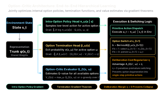
The Option-Critic architecture parameterizes an option $\omega \in \Omega$ with two differentiable neural network heads attached to a shared state representation trunk $\phi(s)$:

1. Intra-Option Policy Head $\pi_{\omega, \theta}(a \mid s)$: A parameterized probability distribution over primitive actions $a \in \mathcal{A}$ conditioned on current state $s$ and active option $\omega$.
2. Termination Function Head $\beta_{\omega, \vartheta}(s)$: A parameterized scalar probability $\beta \in [0, 1]$ (typically generated by a sigmoid activation $\sigma(z_\omega)$) dictating the probability of terminating active option $\omega$ upon entering state $s$.
3. Option Critic Head $Q_\Omega(s, \omega)$: A hierarchical value head estimating the expected return of taking option $\omega$ in state $s$.

1State s_t ──> [ Shared Feature Trunk φ(s_t) ]2                         │3         ┌───────────────┼───────────────┐4         ▼               ▼               ▼5┌─────────────────┐ ┌─────────┐ ┌─────────────────┐6│ Policy π_ω(a|s) │ │ β_ω(s)  │ │ Critic Q_Ω(s,ω) │7│ Action Head     │ │ Exit P  │ │ Option Values   │8└─────────────────┘ └─────────┘ └─────────────────┘9         │               │               │10         ▼               ▼               ▼11      Action a_t    Coin Flip b    Advantage A_Ω12   Execute in Env    (Switch?)      Update Gradients

The Intra-Option Policy Gradient Theorem

Given an active option $\omega$, the intra-option policy parameters $\theta$ are updated to maximize the expected return using the action-value of executing action $a$ under option $\omega$, denoted $Q_U(s, \omega, a)$:

$\frac{\partial Q_\Omega(s, \omega)}{\partial \theta} = \sum_{s', \omega'} \mu_\Omega(s', \omega' \mid s_0, \omega_0) \sum_a \frac{\partial \pi_{\omega', \theta}(a \mid s')}{\partial \theta} Q_U(s', \omega', a)$

where $\mu_\Omega$ represents the discounted state-option visitation distribution, and $Q_U(s, \omega, a)$ is defined recursively through the continuation value $U(s', \omega)$:

$Q_U(s, \omega, a) = r(s, a) + \gamma U(s', \omega)$

The continuation value $U(s', \omega)$ captures the expected value of arriving at state $s'$ under active option $\omega$:

• With probability $(1 - \beta_{\omega, \vartheta}(s'))$, the agent does not terminate and remains in option $\omega$, yielding value $Q_\Omega(s', \omega)$.
• With probability $\beta_{\omega, \vartheta}(s')$, option $\omega$ terminates, allowing the agent to pick a fresh option according to policy over options $\pi_\Omega$, yielding hierarchical state value $V_\Omega(s') = \sum_{\omega'} \pi_\Omega(\omega' \mid s') Q_\Omega(s', \omega')$.

$U(s', \omega) = (1 - \beta_{\omega, \vartheta}(s')) Q_\Omega(s', \omega) + \beta_{\omega, \vartheta}(s') V_\Omega(s')$

The Termination Gradient Theorem

How should the agent adjust the termination parameters $\vartheta$? Bacon et al. showed that the gradient of the expected return with respect to $\vartheta$ depends directly on the Option Advantage function:

$\frac{\partial Q_\Omega(s, \omega)}{\partial \vartheta} = - \sum_{s', \omega'} \mu_\Omega(s', \omega' \mid s_0, \omega_0) \frac{\partial \beta_{\omega', \vartheta}(s')}{\partial \vartheta} A_\Omega(s', \omega')$

where the Option Advantage $A_\Omega(s', \omega)$ measures the relative value of persisting in the current option versus having terminated:

$A_\Omega(s', \omega) = Q_\Omega(s', \omega) - V_\Omega(s')$

Notice the negative sign in the gradient theorem:

• If $Q_\Omega(s', \omega) < V_\Omega(s')$, the current option is underperforming compared to the best available alternative ($A_\Omega < 0$). In this scenario, $-\frac{\partial \beta}{\partial \vartheta} A_\Omega > 0$, so gradient ascent increases $\beta(s')$, encouraging the agent to terminate the sub-optimal option.
• If $Q_\Omega(s', \omega) \ge V_\Omega(s')$, continuing the current option is optimal ($A_\Omega \ge 0$), driving the gradient to decrease $\beta(s')$, maintaining temporal persistence.

Deliberation Cost Regularization

In an unregularized formulation, switching options at every step gives the agent maximal per-step greedy choice. Consequently, without intervention, $\beta(s)$ tends to converge to $1.0$ everywhere, collapsing the options hierarchy into standard single-step flat RL.

To enforce temporal abstraction and penalize needless switching, practitioners introduce a deliberation cost $\eta > 0$ into the termination objective:

$A_{\text{reg}}(s', \omega) = Q_\Omega(s', \omega) - V_\Omega(s') + \eta$

The modified termination update only triggers when the performance deficit of the current option strictly exceeds the switching threshold $\eta$:

$\Delta \vartheta \propto - \frac{\partial \beta_{\omega, \vartheta}(s')}{\partial \vartheta} \left( Q_\Omega(s', \omega) - V_\Omega(s') + \eta \right)$

Worked numerical example

Let us trace a concrete parameter update for the termination head of an Option-Critic agent.

Step 1: Initial State & Values

Suppose an agent transitions to state $s'$ with active option $\omega_1$:

• Available options: $\Omega = \{\omega_1, \omega_2\}$
• Current option value: $Q_\Omega(s', \omega_1) = 4.00$
• Alternative option value: $Q_\Omega(s', \omega_2) = 6.00$
• Hierarchical state value (greedy policy over options): $V_\Omega(s') = \max(4.00, 6.00) = 6.00$

Step 2: Advantage with Deliberation Cost

The raw option advantage is: $A_\Omega(s', \omega_1) = Q_\Omega(s', \omega_1) - V_\Omega(s') = 4.00 - 6.00 = -2.00$

We configure a deliberation cost $\eta = 0.50$: $A_{\text{reg}}(s', \omega_1) = A_\Omega(s', \omega_1) + \eta = -2.00 + 0.50 = -1.50$

Because $A_{\text{reg}} < 0$, staying in option $\omega_1$ is suboptimal even after accounting for the switching penalty.

Step 3: Termination Probability and Gradient

The termination head parameterizes $\beta$ via logit $z$: $\beta = \sigma(z) = \frac{1}{1 + e^{-z}}$

Assume the current logit is $z = 0.00$, yielding: $\beta_{\omega_1}(s') = \sigma(0.00) = \frac{1}{1 + 1} = 0.50$

The derivative of the sigmoid with respect to logit $z$ is: $\frac{\partial \beta}{\partial z} = \beta(1 - \beta) = 0.50 \times (1.00 - 0.50) = 0.25$

The gradient of the regularized return objective with respect to logit $z$ is: $\frac{\partial \mathcal{L}}{\partial z} = \frac{\partial \beta}{\partial z} \cdot A_{\text{reg}} = 0.25 \times (-1.50) = -0.375$

Step 4: Parameter Update

Using learning rate $\alpha = 0.50$, gradient ascent to maximize expected hierarchical return yields: $\Delta z = - \alpha \cdot \frac{\partial \mathcal{L}}{\partial z} = - 0.50 \times (-0.375) = +0.1875$

Updating the logit: $z_{\text{new}} = z + \Delta z = 0.00 + 0.1875 = 0.1875$

Evaluating the new termination probability: $\beta_{\text{new}} = \sigma(0.1875) = \frac{1}{1 + e^{-0.1875}} \approx \frac{1}{1 + 0.8290} \approx 0.5467$

The termination probability increased from $0.5000$ to $0.5467$, correctly incentivizing the agent to abort the inferior option and transition to $\omega_2$.

Code

Below is a self-contained, type-hinted Python implementation verifying the Option Advantage computation, deliberation cost penalty, and termination parameter gradient update.

1import math2from typing import List, Tuple3
4
5def sigmoid(z: float) -> float:6    """Computes standard logistic sigmoid activation."""7    return 1.0 / (1.0 + math.exp(-z))8
9
10class OptionCriticArchitecture:11    """Simulates the Option-Critic architecture, termination gradient theorem, and deliberation cost."""12
13    def __init__(self, deliberation_cost: float = 0.50, alpha: float = 0.50) -> None:14        self.eta = deliberation_cost15        self.alpha = alpha16
17    def compute_option_advantage(18        self, q_current_option: float, all_q_options: List[float]19    ) -> Tuple[float, float, float]:20        """Computes Hierarchical Value V(s'), raw Advantage A(s', omega), and regularized Advantage A_reg.21
22        V(s') = max_omega Q(s', omega).23        A(s', omega) = Q(s', omega) - V(s').24        A_reg = A(s', omega) + eta.25        """26        v_s = max(all_q_options)27        raw_advantage = q_current_option - v_s28        regularized_advantage = raw_advantage + self.eta29        return v_s, raw_advantage, regularized_advantage30
31    def evaluate_termination_gradient_and_update(32        self,33        current_logit_z: float,34        regularized_advantage: float,35    ) -> Tuple[float, float, float, float]:36        """Calculates beta(s'), termination gradient dL/dz, updated logit, and updated beta.37
38        beta = sigmoid(z).39        dL/dz = beta * (1 - beta) * A_reg.40        Delta z = - alpha * dL/dz.41        """42        beta = sigmoid(current_logit_z)43        grad_z = beta * (1.0 - beta) * regularized_advantage44        delta_z = -self.alpha * grad_z45        new_z = current_logit_z + delta_z46        new_beta = sigmoid(new_z)47        return beta, grad_z, new_z, new_beta48
49
50if __name__ == "__main__":51    oc = OptionCriticArchitecture(deliberation_cost=0.50, alpha=0.50)52
53    # State s', options omega_1, omega_254    # Q(s', omega_1) = 4.0, Q(s', omega_2) = 6.055    # Current active option: omega_156    q_omega_1 = 4.057    all_q = [4.0, 6.0]58    z_0 = 0.059
60    v_s, raw_adv, reg_adv = oc.compute_option_advantage(q_omega_1, all_q)61
62    print("=== Option Advantage Calculation ===")63    print(f"Option Q-values:       {all_q}")64    print(f"Hierarchical Value V:  {v_s:.2f} (max Q)")65    print(f"Raw Advantage A:       {raw_adv:.2f} (4.0 - 6.0 = -2.00)")66    print(f"Deliberation Cost eta: {oc.eta:.2f}")67    print(f"Regularized Adv A_reg: {reg_adv:.2f} (-2.00 + 0.50 = -1.50)")68
69    assert math.isclose(v_s, 6.0)70    assert math.isclose(raw_adv, -2.0)71    assert math.isclose(reg_adv, -1.5)72
73    beta_0, grad_z, z_new, beta_new = (74        oc.evaluate_termination_gradient_and_update(z_0, reg_adv)75    )76
77    print("\n=== Termination Gradient & Update ===")78    print(f"Initial logit z:       {z_0:.2f}")79    print(f"Initial beta(s'):      {beta_0:.4f} (sigmoid(0.0) = 0.5000)")80    print(81        f"Gradient dL/dz:        {grad_z:.4f} (0.5 * 0.5 * (-1.50) = -0.3750)"82    )83    print(f"Updated logit z_new:   {z_new:.4f} (0.0 - 0.50 * (-0.375) = +0.1875)")84    print(f"Updated beta_new:      {beta_new:.4f} (sigmoid(0.1875) ≈ 0.5467)")85
86    assert math.isclose(beta_0, 0.50)87    assert math.isclose(grad_z, -0.375)88    assert math.isclose(z_new, 0.1875)89    assert math.isclose(beta_new, 0.546736, rel_tol=1e-4)90    assert beta_new > beta_091
92    print("All Option-Critic assertions passed successfully!")

Expected output:

1=== Option Advantage Calculation ===2Option Q-values:       [4.0, 6.0]3Hierarchical Value V:  6.00 (max Q)4Raw Advantage A:       -2.00 (4.0 - 6.0 = -2.00)5Deliberation Cost eta: 0.506Regularized Adv A_reg: -1.50 (-2.00 + 0.50 = -1.50)7
8=== Termination Gradient & Update ===9Initial logit z:       0.0010Initial beta(s'):      0.5000 (sigmoid(0.0) = 0.5000)11Gradient dL/dz:        -0.3750 (0.5 * 0.5 * (-1.50) = -0.3750)12Updated logit z_new:   0.1875 (0.0 - 0.50 * (-0.375) = +0.1875)13Updated beta_new:      0.5467 (sigmoid(0.1875) ≈ 0.5467)14All Option-Critic assertions passed successfully!

Watch Out For

The Quick Version

• End-to-End Discovery: Option-Critic replaces manual subgoal and option engineering by jointly learning intra-option policies $\pi_\omega$, termination probabilities $\beta_\omega$, and value functions $Q_\Omega$ via gradient theorems.
• Intra-Option Policy Gradient: Updates internal primitive action policies $\pi_\omega(a \mid s)$ using the augmented state-option-action value $Q_U(s, \omega, a)$, weighting actions that maximize long-term option utility.
• Termination Gradient Theorem: Updates option stopping probability $\beta_\omega(s)$ proportionally to the option advantage $Q_\Omega(s', \omega) - V_\Omega(s')$, naturally triggering termination when the current option becomes suboptimal.
• Deliberation Cost Margin: To prevent options from collapsing into single-step actions ($\beta \to 1$), a deliberation cost penalty $\eta > 0$ is added to the advantage, enforcing temporal persistence and meaningful macro-actions.

What to Read Next

• The Options Framework
• Hierarchical RL
• Feudal Networks (FuN)