The Options Framework

The Options Framework extends reinforcement learning beyond single-step primitive actions by formalizing temporally extended subroutines with initiation sets, internal policies, and termination conditions.

Why Does This Exist?

In standard reinforcement learning, the agent operates in lockstep with a discrete clock: at every single timestep $t$ , the agent receives state $s_t$ , selects a single primitive action $a_t$ , receives reward $r_{t+1}$ , and transitions to $s_{t+1}$ . For complex, long-horizon tasks—such as an autonomous robot navigating across an entire office building or solving an intricate manipulation puzzle—this flat, step-by-step representation introduces severe bottlenecks:

Exponential Exploration Complexity: If an agent must take 10,000 primitive joint motor commands to reach a distant room, undirected random exploration (like $\epsilon$ -greedy) requires exponential time to stumble upon the goal. The probability of randomly generating a coherent sequence of thousands of low-level motor torques is virtually zero.
Diluted Credit Assignment: When a delayed reward is finally discovered after thousands of steps, Temporal Difference Learning must backpropagate that reward signal backwards across thousands of individual transitions, requiring millions of training iterations for values to propagate to initial states.
Inability to Reuse Behavioral Modules: Biological intelligence does not plan at the millisecond motor-twitch level. When deciding to grab a cup of coffee, humans invoke macro-behaviors: "stand up", "walk down the hall", "open door", and "grasp cup". Flat RL forces the agent to relearn basic locomotion primitives from scratch for every new task.

The Options Framework, formalized in the seminal work of Richard Sutton, Doina Precup, and Satinder Singh (1999), resolves this by bringing temporal abstraction to reinforcement learning. Instead of restricting actions to single-step primitives, the framework formalizes macro-actions—termed options—that execute over variable temporal durations. By embedding options into the mathematics of Semi-Markov Decision Processes (SMDPs), the framework allows agents to plan, learn, and act seamlessly across multiple time scales without abandoning the rigorous convergence guarantees of dynamic programming.

Think of It Like This

Reusable Subroutines in Software Engineering

Imagine writing a complex software application in raw x86 assembly language where your only available operations are single-clock-cycle CPU instructions: bit-shifts, register increments, and jumps.

If you had to write every sorting algorithm, network socket connection, and file reading loop by copy-pasting hundreds of lines of assembly instructions directly into your main() loop, programming would be impossible. Finding bugs would be agonizing, and optimizing high-level business logic would get lost in the weeds of register allocation.

Instead, computer science relies on functions and subroutines:

A function like quicksort(array) has a clear entry prerequisite: the input must be an array of comparable items (the Initiation Set).
Once invoked, the function executes a specialized sequence of loops and swaps across hundreds or thousands of CPU cycles (the Internal Policy).
When the array is fully partitioned and sorted, the function reaches a return statement and exits (the Termination Condition).

At the high-level application level, your program simply calls quicksort(). The CPU still executes primitive assembly instructions underneath, but your planning logic operates across macro-level units of work.

The Options Framework does the exact same thing for reinforcement learning agents. An option is a callable behavioral subroutine: the agent invokes a high-level option like navigate_to_doorway(), the option runs its internal policy for $k$ environment ticks, and returns control to the high-level policy when the doorway is reached.

Where the analogy stops: Software subroutines are typically deterministic and write to clean memory addresses. In RL, options operate in stochastic, partially observable physical environments, where transitions are probabilistic and termination conditions $\beta_\omega(s)$ are stochastic functions evaluated at every state.

How It Actually Works

Formal 3-Tuple Definition of an Option

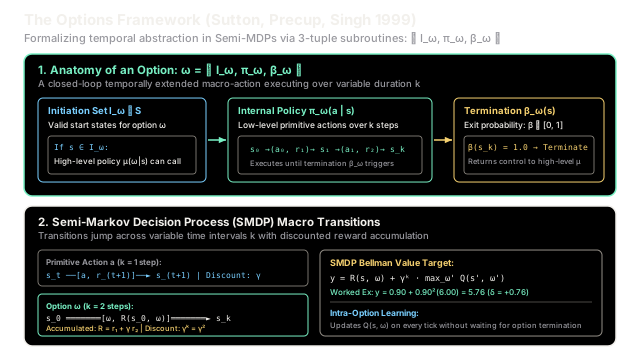
In the Options Framework, an option $\omega \in \Omega$ is formally defined as a 3-tuple:

\omega = \langle \mathcal{I}_\omega, \pi_\omega, \beta_\omega \rangle

where:

Initiation Set $\mathcal{I}_\omega \subseteq \mathcal{S}$ : The subset of states in which the option can be initiated. An option $\omega$ is available to be selected at state $s$ if and only if $s \in \mathcal{I}_\omega$ . The set of available options at state $s$ is denoted $\Omega(s) = \{\omega \in \Omega \mid s \in \mathcal{I}_\omega\}$ .
Internal Policy $\pi_\omega: \mathcal{S} \times \mathcal{A} \to [0, 1]$ : The policy governing the agent while option $\omega$ is executing. When in state $s$ under active option $\omega$ , the agent selects primitive action $a$ with probability $\pi_\omega(a | s)$ .
Termination Condition $\beta_\omega: \mathcal{S} \to [0, 1]$ : A function giving the probability that the option terminates upon arriving in state $s$ . If the agent enters state $s$ , option $\omega$ terminates with probability $\beta_\omega(s)$ , relinquishing control back to the high-level policy. With probability $1 - \beta_\omega(s)$ , the option continues executing $\pi_\omega$ .

Primitive Actions as Degenerate Options:
Every standard primitive action $a \in \mathcal{A}$ can be expressed as a 1-step option:

\mathcal{I}_a = \mathcal{S}, \quad \pi_a(a' | s) = \mathbb{I}(a' = a), \quad \beta_a(s) = 1.0, \quad \forall s \in \mathcal{S}

Because primitive actions are valid options of duration $k = 1$ , an agent utilizing the options framework retains the full expressive capacity of the original MDP.

Semi-Markov Decision Processes (SMDPs) and Intra-Option Learning

When an agent selects among options that execute over variable temporal durations $k \in \{1, 2, 3, \dots\}$ , the underlying discrete-time Markov Decision Process transitions to a Semi-Markov Decision Process (SMDP) at the macro level.

1Primitive MDP (k = 1):2s_0 ──[a_0, r_1]──► s_1 ──[a_1, r_2]──► s_2 ──[a_2, r_3]──► s_3 (Discount: gamma)3
4Macro SMDP (k = 3 steps):5s_0 ═══════════════[ Option omega, R(s_0, omega) ]══════════════► s_3 (Discount: gamma^3)6    (Executes internal policy pi_omega until beta_omega(s_3) = 1)

1. SMDP Reward and Transition Models

Let $\mathcal{E}(s, \omega)$ denote the event that option $\omega$ is initiated at state $s$ at time $t$ , terminating at time $t+k$ in state $s'$ .

The expected multi-step discounted reward of option $\omega$ is:

R(s, \omega) = \mathbb{E} \left[ r_{t+1} + \gamma r_{t+2} + \gamma^2 r_{t+3} + \dots + \gamma^{k-1} r_{t+k} \,\Big|\, \mathcal{E}(s, \omega) \right]

The discounted transition probability to arrive at terminal state $s'$ under option $\omega$ across all possible durations $k$ is:

P(s' \mid s, \omega) = \sum_{k=1}^\infty \gamma^k P(s', k \mid s, \omega)

where $P(s', k \mid s, \omega)$ is the joint probability that option $\omega$ terminates in state $s'$ after exactly $k$ steps.

2. Macro-Level Bellman Equations over Options

Let $\mu(\omega | s)$ denote the high-level policy over options, which selects which option to execute upon option termination. The action-value of executing option $\omega$ in state $s$ satisfies the Bellman Equation:

Q(s, \omega) = R(s, \omega) + \sum_{s' \in \mathcal{S}} P(s' \mid s, \omega) \max_{\omega' \in \Omega(s')} Q(s', \omega')

The optimal state value across all available options is:

V^*(s) = \max_{\omega \in \Omega(s)} Q^*(s, \omega)

3. Intra-Option Learning

Standard SMDP Q-learning waits until an option fully terminates after $k$ steps before performing a single value update. If an option executes for 50 steps, nothing is learned until step 50.

Intra-Option Learning overcomes this latency by updating option values on every single primitive transition $(s, a, r, s')$ :

Q(s, \omega) \leftarrow Q(s, \omega) + \alpha \left[ r + \gamma U(s', \omega) - Q(s, \omega) \right]

where $U(s', \omega)$ represents the expected value of arriving in state $s'$ :

U(s', \omega) = (1 - \beta_\omega(s')) Q(s', \omega) + \beta_\omega(s') \max_{\omega' \in \Omega(s')} Q(s', \omega')

If the option continues ( $\beta_\omega(s') = 0$ ), the bootstrap target is $Q(s', \omega)$ . If the option terminates ( $\beta_\omega(s') = 1$ ), the target switches to the optimal next option value $\max_{\omega'} Q(s', \omega')$ . Crucially, intra-option learning enables off-option learning: an experience tuple generated by one option can simultaneously update all other options whose internal policy is consistent with action $a$ .

Worked numerical example

Let us trace a concrete option execution in the classic 4-room gridworld door navigation problem:

Environment Setup:
- State $s_0$ : Interior room position (non-terminal). Current option estimate: $Q(s_0, \omega_{\text{door}}) = 5.00$ .
- State $s_1$ : Intermediate hallway position.
- State $s_2 = s_{\text{door}}$ : Goal doorway connecting Room 1 to Room 2.
Option $\omega_{\text{door}}$ Specification:
- Initiation set: $\mathcal{I}_{\text{door}} = \text{Room 1 states}$ .
- Termination condition:
  - $\beta(s_1) = 0.0$ (continue).
  - $\beta(s_2) = 1.0$ (terminate at doorway).
- Discount factor: $\gamma = 0.90$ .
Option Trajectory Rollout ( $k = 2$ primitive steps):
- Step 1: Takes primitive action $a_0 = \text{East}$ , receives reward $r_1 = 0.0$ , reaches $s_1$ . Termination check: $\beta(s_1) = 0.0$ .
- Step 2: Takes primitive action $a_1 = \text{East}$ , receives reward $r_2 = +1.0$ , reaches doorway $s_2$ . Termination check: $\beta(s_2) = 1.0 \implies$ Option terminates!
Next-State Value:
- At doorway $s_2$ , the agent can invoke options to enter Room 2. Suppose maximum next option value is: $\max_{\omega' \in \Omega(s_2)} Q(s_2, \omega') = 6.00$

Step 1: Compute the Multi-Step Discounted Reward $R(s_0, \omega_{\text{door}})$

The accumulated discounted reward over the duration $k = 2$ is:

R(s_0, \omega_{\text{door}}) = r_1 + \gamma r_2 = 0.0 + 0.90 \times 1.0 = 0.90

Step 2: Compute the Effective Temporal Discount Factor

Because the option executed for $k = 2$ primitive timesteps, the future value at termination is discounted by $\gamma^k$ :

\gamma^k = \gamma^2 = (0.90)^2 = 0.81

Step 3: Compute the SMDP Bellman Target

The SMDP Bellman target for option value $Q(s_0, \omega_{\text{door}})$ is:

y_{\text{SMDP}} = R(s_0, \omega_{\text{door}}) + \gamma^k \max_{\omega' \in \Omega(s_2)} Q(s_2, \omega') = 0.90 + 0.81 \times 6.00 = 0.90 + 4.86 = 5.76

Step 4: Evaluate Temporal Difference (TD) Error and Loss

Compared against the prior estimate $Q(s_0, \omega_{\text{door}}) = 5.00$ :

\delta_{\text{SMDP}} = y_{\text{SMDP}} - Q(s_0, \omega_{\text{door}}) = 5.76 - 5.00 = +0.76

The squared Bellman error loss is:

\mathcal{L} = \frac{1}{2} \delta^2 = \frac{1}{2} (0.76)^2 = \frac{1}{2} \times 0.5776 = 0.2888

Step 5: Contrast with Intra-Option Evaluation at Step 2

Under intra-option learning at step 2 (transition from $s_1 \to s_2$ with $r = 1.0$ and $\beta(s_2) = 1.0$ ):

y_{\text{intra}} = r_2 + \gamma \left[ (1 - \beta(s_2)) Q(s_2, \omega) + \beta(s_2) \max_{\omega'} Q(s_2, \omega') \right]

y_{\text{intra}} = 1.0 + 0.90 \left[ (0.0) + (1.0 \times 6.00) \right] = 1.0 + 0.90 \times 6.00 = 6.40

Intra-option learning updates the value of reaching the doorway immediately on step 2 without waiting for retrospective SMDP trajectory stitching.

Code

1import numpy as np2
3
4class OptionsFrameworkEvaluator:5    """Evaluates multi-step temporal abstraction under the Options Framework:6
7    Option 3-tuple <I, pi, beta>, SMDP discounted return integration,8    macro-Bellman target computation, and intra-option TD updates.9    """10
11    def __init__(self, gamma: float = 0.90) -> None:12        self.gamma = gamma13
14    def compute_smdp_return(15        self, step_rewards: list[float]16    ) -> tuple[float, float, int]:17        """Computes multi-step discounted SMDP reward R(s, omega) and effective discount gamma^k:18
19        R(s, omega) = sum_{t=0}^{k-1} gamma^t * r_{t+1}20        """21        k = len(step_rewards)22        discounted_r = 0.023        for t, r in enumerate(step_rewards):24            discounted_r += (self.gamma**t) * r25        effective_gamma = self.gamma**k26        return float(discounted_r), float(effective_gamma), k27
28    def compute_smdp_target(29        self,30        smdp_return: float,31        effective_gamma: float,32        next_state_max_q: float,33    ) -> float:34        """Computes SMDP Bellman target: y = R(s, omega) + gamma^k * max_{omega'} Q(s', omega')."""35        return float(smdp_return + effective_gamma * next_state_max_q)36
37    def compute_intra_option_target(38        self,39        reward: float,40        beta_next: float,41        q_same_option: float,42        next_max_q: float,43    ) -> float:44        """Computes single-step intra-option target:45
46        y_intra = r + gamma * [ (1 - beta(s')) * Q(s', omega) + beta(s') * max_{omega'} Q(s', omega') ]47        """48        expected_continuation = (49            1.0 - beta_next50        ) * q_same_option + beta_next * next_max_q51        return float(reward + self.gamma * expected_continuation)52
53
54if __name__ == "__main__":55    np.set_printoptions(precision=4, suppress=True)56
57    evaluator = OptionsFrameworkEvaluator(gamma=0.90)58
59    # 4-room gridworld door navigation worked example60    # Step 1: r=0.0, s1, beta(s1)=0.061    # Step 2: r=1.0, s2=s_door, beta(s2)=1.062    step_rewards = [0.0, 1.0]63    next_max_q = 6.0064    current_q_s0 = 5.0065
66    # 1. SMDP multi-step return and effective discount67    r_smdp, eff_gamma, duration = evaluator.compute_smdp_return(step_rewards)68
69    # 2. SMDP Bellman target and temporal difference error70    target_smdp = evaluator.compute_smdp_target(r_smdp, eff_gamma, next_max_q)71    td_error_smdp = target_smdp - current_q_s072    loss_smdp = 0.5 * (td_error_smdp**2)73
74    # 3. Step-by-step intra-option targets75    # Step 1: r=0.0, arrives at s1 where beta=0.0, suppose Q(s1, omega)=5.5076    y_intra_step1 = evaluator.compute_intra_option_target(77        reward=0.0, beta_next=0.0, q_same_option=5.50, next_max_q=5.5078    )79    # Step 2: r=1.0, arrives at s2 where beta=1.0, next_max_q=6.0080    y_intra_step2 = evaluator.compute_intra_option_target(81        reward=1.0, beta_next=1.0, q_same_option=4.00, next_max_q=6.0082    )83
84    print(f"Option Duration k: {duration} steps")85    # -> Option Duration k: 2 steps86
87    print(f"SMDP Multi-Step Reward R(s_0, omega): {r_smdp:.2f}")88    # -> SMDP Multi-Step Reward R(s_0, omega): 0.9089
90    print(f"Effective Discount gamma^k: {eff_gamma:.4f}")91    # -> Effective Discount gamma^k: 0.810092
93    print(f"SMDP Bellman Target y: {target_smdp:.2f}")94    # -> SMDP Bellman Target y: 5.7695
96    print(f"SMDP TD Error delta: +{td_error_smdp:.2f}")97    # -> SMDP TD Error delta: +0.7698
99    print(f"Squared Bellman Loss: {loss_smdp:.4f}")100    # -> Squared Bellman Loss: 0.2888101
102    print(f"Intra-Option Step 1 Target: {y_intra_step1:.2f}")103    # -> Intra-Option Step 1 Target: 4.95104
105    print(f"Intra-Option Step 2 Target: {y_intra_step2:.2f}")106    # -> Intra-Option Step 2 Target: 6.40107
108    # Assert correctness against worked example values109    assert duration == 2110    assert np.isclose(r_smdp, 0.90, atol=1e-2)111    assert np.isclose(eff_gamma, 0.81, atol=1e-2)112    assert np.isclose(target_smdp, 5.76, atol=1e-2)113    assert np.isclose(td_error_smdp, 0.76, atol=1e-2)114    assert np.isclose(loss_smdp, 0.2888, atol=1e-3)115    assert np.isclose(y_intra_step1, 4.95, atol=1e-2)116    assert np.isclose(y_intra_step2, 6.40, atol=1e-2)

Watch Out For

Option Degeneration, Chattering, and the Curse of Handcrafted Abstractions

When implementing hierarchical systems using the Options Framework, practitioners frequently encounter two catastrophic failure modes related to the termination condition $\beta_\omega$ :

Option Chattering (Premature Termination): If termination functions $\beta_\omega(s)$ are set too liberally (e.g., terminating whenever minor noise occurs), the high-level policy switches options at almost every timestep ( $k = 1$ ). This destroys the entire benefit of temporal abstraction, reverting the SMDP back into a flat, high-variance MDP while adding the computational overhead of hierarchical evaluation.
Option Degeneration (Zombie Options): Conversely, if termination conditions are too strict or internal policies get stuck in loops, an option may never terminate ( $k \to \infty$ ). The high-level policy is locked out of control, unable to adapt if environmental conditions shift.
The Sub-Optimality Gap: Manually handcrafting options (e.g., hardcoding doorway waypoints) biases the agent's state-visitation trajectory. If the handcrafted subroutines fail to capture the true optimal path, the hierarchically optimal policy $\mu^*$ will strictly underperform a flat, unconstrained policy.

The Fix: Modern hierarchical RL moves away from static, hand-designed options and uses end-to-end option discovery:

Adopt the Option-Critic Architecture, which parameterizes the termination function $\beta_\omega(s; \vartheta)$ as a differentiable neural network trained directly via policy gradients to terminate only when the option's continuation value falls below the value of switching options.
Incorporate a deliberation cost (or switching penalty) $\eta > 0$ into the termination gradient: penalize frequent option switching to naturally encourage longer, temporally meaningful options without manual tuning.

The Quick Version

Temporal Abstraction 3-Tuple: An option $\omega = \langle \mathcal{I}_\omega, \pi_\omega, \beta_\omega \rangle$ formalizes macro-behaviors through an initiation set $\mathcal{I}_\omega$ , an internal primitive policy $\pi_\omega$ , and a termination condition $\beta_\omega$ .
Semi-Markov Decision Process (SMDP): When options execute over variable durations $k \ge 1$ , the macro-level transition dynamics form an SMDP where rewards accumulate as $R(s, \omega) = \sum_{t=0}^{k-1} \gamma^t r_{t+1}$ and future values discount by $\gamma^k$ .
Intra-Option Efficiency: Intra-option learning avoids waiting for an option to terminate after $k$ steps by updating option action-values on every primitive transition, enabling simultaneous off-option updates.
Overcoming Flat RL Limits: Options dramatically accelerate exploration and credit assignment in long-horizon sparse-reward environments, serving as the foundational building block for modern hierarchical RL architectures like Option-Critic and Feudal Networks.