Rainbow DQN

Why Does This Exist?

Between the publication of the original Deep Q-Network (DQN) in 2015 and 2017, the deep reinforcement learning community developed several distinct, highly successful enhancements to address specific algorithmic weaknesses in DQN:

• Double DQN addressed the maximization bias that causes runaway overestimation of action values.
• Prioritized Experience Replay (PER) replaced uniform transition replay with priority sampling proportional to temporal difference error magnitude, dramatically boosting data efficiency.
• Dueling Networks decomposed state-action values into state values and action advantages, accelerating policy evaluation in states where action choice has negligible impact.
• Multi-Step Learning ($n$-step returns) expanded the temporal horizon of bootstrapping to balance variance against bias and propagate sparse rewards faster.
• Distributional RL (Categorical DQN / C51) replaced scalar expected value predictions with full probability distributions over return support atoms, stabilizing gradient signals.
• Noisy Nets eliminated manual $\epsilon$-greedy schedules in favor of learnable parametric noise added directly to network weights.

While each method improved performance in isolation, researchers did not know whether these techniques were mutually compatible. Would combining them create harmful interference? Would the variance of multi-step bootstrapping corrupt categorical distribution projections? Would prioritized replay destabilize noisy linear layers?

In 2018, Matteo Hessel and researchers at DeepMind answered these questions by introducing Rainbow DQN. They demonstrated not only that all six extensions could be combined harmoniously, but that their mathematical interactions are deeply synergistic. Rainbow set a historic benchmark on the Atari 2600 suite, outperforming every individual component by a wide margin in both data efficiency and asymptotic policy score.

Think of It Like This

How It Actually Works

The Six Integrated Pillars

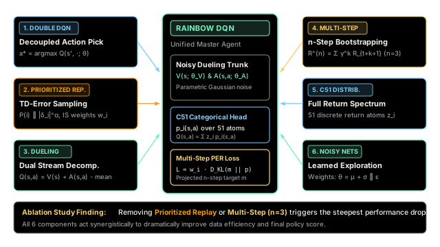
Rainbow DQN synthesizes six foundational extensions into a single unified agent:

1                          ┌────────────────────────┐2                          │   1. Double Q-Learning  │3                          │  Decoupled Action Pick │4                          └───────────┬────────────┘5                                      │6┌────────────────────────┐            ▼            ┌────────────────────────┐7│  2. Prioritized Replay │──►  RAINBOW DQN HUB  ◄──│  4. Multi-Step (n=3)   │8│   Sampling via |TD|^α  │     Unified Master      │   Accelerated Rewards  │9└────────────────────────┘          Agent          └────────────────────────┘10                                      ▲11                                      │12                          ┌───────────┴────────────┐13                          │ 3. Dueling Streams     │14                          │ 5. Distributional C51  │15                          │ 6. Noisy Linear Layers │16                          └────────────────────────┘

1. Double Q-Learning (DDQN)

Standard Q-learning uses the target network for both selecting and evaluating the best next action: $\max_a Q(S_{t+1}, a; \theta^-)$. This introduces severe maximization bias. Double DQN decouples these two roles: the online network selects the greedy action, while the target network evaluates its value: $a^* = \arg\max_{a} Q(S_{t+n}, a; \theta)$ $y_t = R_t^{(n)} + \gamma^n Q(S_{t+n}, a^*; \theta^-)$

In Rainbow's distributional context, the greedy action is selected by maximizing the expectation over the online network's distribution: $a^* = \arg\max_a \sum_{i} z_i \, p_i(S_{t+n}, a; \theta)$

2. Prioritized Experience Replay (PER)

Rather than sampling transitions uniformly from the replay buffer, PER samples transitions with probability proportional to their priority: $P(k) = \frac{p_k^\alpha}{\sum_j p_j^\alpha}$ where $p_k$ is the Kullback-Leibler (KL) divergence or temporal difference error of transition $k$, and $\alpha$ controls the degree of prioritization. To correct for the non-uniform sampling bias, updates are weighted by importance sampling (IS) weights: $w_k = \left(\frac{1}{N \cdot P(k)}\right)^\beta \Bigg/ \max_j w_j$ where $\beta$ is annealed from $\beta_0 \approx 0.4$ up to $1.0$ over training.

3. Dueling Network Architecture

The neural representation splits into two distinct streams after a shared convolutional/dense trunk:

• A scalar Value stream $V(s)$ estimating the general goodness of the state.
• An Advantage stream $A(s, a)$ estimating the relative benefit of each action.

In Rainbow, both streams output logit distributions over the $N_{\text{atoms}}$ support atoms. For each atom $i \in \{0, \dots, N_{\text{atoms}}-1\}$: $q_i(s, a) = V_i(s) + \left(A_i(s, a) - \frac{1}{|\mathcal{A}|} \sum_{a' \in \mathcal{A}} A_i(s, a')\right)$ The probabilities are obtained via softmax over the atom dimension: $p_i(s, a) = \frac{\exp(q_i(s, a))}{\sum_{j} \exp(q_j(s, a))}$

4. Multi-Step Learning ($n=3$)

Rather than bootstrapping immediately from $S_{t+1}$, Rainbow accumulates discounted rewards over an $n$-step horizon (standard default: $n=3$): $R_t^{(n)} \triangleq \sum_{k=0}^{n-1} \gamma^k R_{t+k+1}$ The target then bootstraps from state $S_{t+n}$ discounted by $\gamma^n$: $\hat{T}^{(n)} z_j = R_t^{(n)} + \gamma^n z_j$ This dramatically accelerates the propagation of delayed rewards while reducing temporal difference bias.

5. Distributional Reinforcement Learning (C51)

Instead of predicting a single expected scalar $Q(s, a)$, the network models the full return distribution as a categorical distribution over $N_{\text{atoms}} = 51$ fixed, equally spaced support atoms: $\mathcal{Z} = \{z_i = V_{\min} + i \cdot \Delta z \mid i = 0, \dots, N_{\text{atoms}}-1\}, \quad \Delta z = \frac{V_{\max} - V_{\min}}{N_{\text{atoms}} - 1}$ The shifted return $\hat{T}^{(n)} z_j$ is clipped to $[V_{\min}, V_{\max}]$ and projected onto neighboring atoms $l = \lfloor b_j \rfloor$ and $u = \lceil b_j \rceil$ via linear interpolation, accumulating projected target distribution $\mathbf{m}$: $b_j = \frac{\text{clip}(\hat{T}^{(n)} z_j, V_{\min}, V_{\max}) - V_{\min}}{\Delta z}$ $m_l \mathrel{+}= p_j(S_{t+n}, a^*; \theta^-) \cdot (u - b_j), \quad m_u \mathrel{+}= p_j(S_{t+n}, a^*; \theta^-) \cdot (b_j - l)$

6. Noisy Nets for Exploration

Rainbow replaces manual $\epsilon$-greedy exploration with NoisyLinear layers in both the value and advantage heads. Each linear layer replaces fixed weight matrix $\mathbf{W}$ and bias $\mathbf{b}$ with: $\mathbf{W} = \boldsymbol{\mu}^W + \boldsymbol{\sigma}^W \odot \boldsymbol{\varepsilon}^W, \quad \mathbf{b} = \boldsymbol{\mu}^b + \boldsymbol{\sigma}^b \odot \boldsymbol{\varepsilon}^b$ where $\boldsymbol{\mu}$ and $\boldsymbol{\sigma}$ are learnable parameters, and $\boldsymbol{\varepsilon}$ is stochastic noise drawn from a factorized Gaussian distribution. The network learns to modulate its own exploration rates across different states.

The Unified Master Loss

Rainbow combines all six components into a single objective function: the Kullback-Leibler divergence (categorical cross-entropy) between the multi-step projected target distribution $\mathbf{m}_t^{(n)}$ and the online network's predicted distribution $\mathbf{p}(S_t, A_t; \theta)$, weighted by PER importance sampling weights:

$\mathcal{L}_{\text{Rainbow}}(\theta) = \sum_{t} w_t \, D_{\text{KL}}\left(\mathbf{m}_t^{(n)} \parallel \mathbf{p}(S_t, A_t; \theta)\right) = -\sum_{t} w_t \sum_{i=0}^{N_{\text{atoms}}-1} m_{t, i}^{(n)} \log p_i(S_t, A_t; \theta)$

The transition priority stored in the PER buffer is updated directly with the KL divergence: $p_t \leftarrow D_{\text{KL}}\left(\mathbf{m}_t^{(n)} \parallel \mathbf{p}(S_t, A_t; \theta)\right) + \epsilon_{\text{PER}}$

Findings from the Rainbow Ablation Study

In their seminal ablation experiment, Hessel et al. systematically removed one component at a time from Rainbow to evaluate its relative contribution:

The study revealed a critical insight: Prioritized Experience Replay and Multi-Step Learning are the two most indispensable pillars of Rainbow DQN. Removing either one causes immediate performance degradation.

Worked numerical example

Let us trace a single multi-step distributional target calculation and PER-weighted loss update on a simplified 5-atom system:

• Number of atoms: $N_{\text{atoms}} = 5$
• Bounds: $V_{\min} = 0.0, V_{\max} = 8.0$
• Atom step: $\Delta z = \frac{8.0 - 0.0}{5 - 1} = 2.0$
• Support atoms: $\mathcal{Z} = [0.0, 2.0, 4.0, 6.0, 8.0]$
• Discount factor: $\gamma = 0.9$, multi-step horizon $n = 3 \implies \gamma^3 = 0.729$
• Observed 3-step rewards: $R_1 = 1.0, R_2 = 0.0, R_3 = 2.0$
• Accumulated return: $R^{(3)} = R_1 + \gamma R_2 + \gamma^2 R_3 = 1.0 + 0.9(0.0) + 0.81(2.0) = 1.0 + 1.62 = 2.62$
• Target network distribution for Double-DQN greedy action $a^*$: $\mathbf{p}(S_{t+3}, a^*; \theta^-) = [0.10, 0.20, 0.40, 0.20, 0.10]^\top$
• PER importance sampling weight: $w = 0.85$

Step 1: Shift and project each atom $z_j$

For each support atom $z_j$, compute shifted value $\hat{T} z_j = R^{(3)} + \gamma^3 z_j$, clip to $[0.0, 8.0]$, find coordinate $b_j = \hat{T} z_j / \Delta z$, and project onto $l = \lfloor b_j \rfloor$ and $u = \lceil b_j \rceil$:

1. Atom $j=0$ ($z_0 = 0.0$): $\hat{T} z_0 = 2.62 + 0.729(0.0) = 2.62 \implies b_0 = 2.62 / 2.0 = 1.31 \implies l=1, u=2$

   • Contrib to $m_1$: $p_0 \times (2 - 1.31) = 0.10 \times 0.69 = 0.0690$
   • Contrib to $m_2$: $p_0 \times (1.31 - 1) = 0.10 \times 0.31 = 0.0310$

2. Atom $j=1$ ($z_1 = 2.0$): $\hat{T} z_1 = 2.62 + 0.729(2.0) = 4.078 \implies b_1 = 4.078 / 2.0 = 2.039 \implies l=2, u=3$

   • Contrib to $m_2$: $p_1 \times (3 - 2.039) = 0.20 \times 0.961 = 0.1922$
   • Contrib to $m_3$: $p_1 \times (2.039 - 2) = 0.20 \times 0.039 = 0.0078$

3. Atom $j=2$ ($z_2 = 4.0$): $\hat{T} z_2 = 2.62 + 0.729(4.0) = 5.536 \implies b_2 = 5.536 / 2.0 = 2.768 \implies l=2, u=3$

   • Contrib to $m_2$: $p_2 \times (3 - 2.768) = 0.40 \times 0.232 = 0.0928$
   • Contrib to $m_3$: $p_2 \times (2.768 - 2) = 0.40 \times 0.768 = 0.3072$

4. Atom $j=3$ ($z_3 = 6.0$): $\hat{T} z_3 = 2.62 + 0.729(6.0) = 6.994 \implies b_3 = 6.994 / 2.0 = 3.497 \implies l=3, u=4$

   • Contrib to $m_3$: $p_3 \times (4 - 3.497) = 0.20 \times 0.503 = 0.1006$
   • Contrib to $m_4$: $p_3 \times (3.497 - 3) = 0.20 \times 0.497 = 0.0994$

5. Atom $j=4$ ($z_4 = 8.0$): $\hat{T} z_4 = \text{clip}(2.62 + 0.729(8.0), 0, 8) = \text{clip}(8.452, 0, 8) = 8.0 \implies b_4 = 4.0 \implies l=4, u=4$

   • Contrib to $m_4$: $p_4 \times 1.0 = 0.1000$

Step 2: Sum the projected target probabilities

$m_0 = 0.0000$ $m_1 = 0.0690$ $m_2 = 0.0310 + 0.1922 + 0.0928 = 0.3160$ $m_3 = 0.0078 + 0.3072 + 0.1006 = 0.4156$ $m_4 = 0.0994 + 0.1000 = 0.1994$ $\sum_{i=0}^4 m_i = 0.0 + 0.0690 + 0.3160 + 0.4156 + 0.1994 = 1.0000$

Step 3: Compute Cross-Entropy and PER-Weighted Loss

Suppose the online network's current predicted distribution is $\mathbf{p}(S_t, A_t; \theta) = [0.20, 0.30, 0.30, 0.10, 0.10]^\top$.

Compute the cross-entropy: $\mathcal{L}_{\text{CE}} = -\sum_{i=0}^4 m_i \log p_i$ $\mathcal{L}_{\text{CE}} = -\Big[0 + 0.0690 \ln(0.30) + 0.3160 \ln(0.30) + 0.4156 \ln(0.10) + 0.1994 \ln(0.10)\Big]$ $\mathcal{L}_{\text{CE}} = -\Big[0.0690(-1.20397) + 0.3160(-1.20397) + 0.4156(-2.30259) + 0.1994(-2.30259)\Big]$ $\mathcal{L}_{\text{CE}} = -(-0.08307 - 0.38045 - 0.95696 - 0.45914) = 1.8796$

Scale by the PER importance sampling weight $w = 0.85$: $\mathcal{L}_{\text{Rainbow}} = w \cdot \mathcal{L}_{\text{CE}} = 0.85 \times 1.8796 = 1.5977$

Code

The following self-contained Python implementation constructs the complete Rainbow DQN core modules: a factorized NoisyLinear layer, a Dueling C51 categorical network, and the Multi-Step Double DQN target projection with PER weighting:

1"""Self-contained implementation of the Rainbow DQN core architecture.2
3Integrates:41. NoisyLinear layers (factorized Gaussian exploration)52. Dueling Network architecture (decoupled Value and Advantage streams)63. Distributional RL (Categorical C51 projection)74. Double Q-learning (decoupled greedy action selection)85. Multi-Step Returns (n-step accumulated target projection)96. Prioritized Experience Replay (importance-weighted cross-entropy loss)10"""11
12from typing import Dict, Tuple13import numpy as np14
15
16class NoisyLinear:17    """Factorized Gaussian Noisy Linear Layer for parametric exploration."""18
19    def __init__(20        self,21        in_features: int,22        out_features: int,23        sigma_init: float = 0.5,24        seed: int = 4225    ) -> None:26        np.random.seed(seed)27        self.in_features: int = in_features28        self.out_features: int = out_features29
30        val: float = 1.0 / np.sqrt(in_features)31        self.weight_mu: np.ndarray = np.random.uniform(-val, val, (out_features, in_features))32        self.weight_sigma: np.ndarray = np.full((out_features, in_features), sigma_init / np.sqrt(in_features))33
34        self.bias_mu: np.ndarray = np.random.uniform(-val, val, out_features)35        self.bias_sigma: np.ndarray = np.full(out_features, sigma_init / np.sqrt(out_features))36
37    @staticmethod38    def _scale_noise(size: int) -> np.ndarray:39        x = np.random.randn(size)40        return np.sign(x) * np.sqrt(np.abs(x))41
42    def forward(self, x: np.ndarray, train: bool = True) -> np.ndarray:43        """Forward pass sampling factorized Gaussian noise when train=True."""44        if train:45            p_in = self._scale_noise(self.in_features)46            p_out = self._scale_noise(self.out_features)47            w_eps = np.outer(p_out, p_in)48            b_eps = p_out49            w = self.weight_mu + self.weight_sigma * w_eps50            b = self.bias_mu + self.bias_sigma * b_eps51        else:52            w = self.weight_mu53            b = self.bias_mu54        return x @ w.T + b55
56
57class RainbowDuelingC51:58    """Dueling Distributional (C51) Network with Noisy Linear layers."""59
60    def __init__(61        self,62        state_dim: int = 4,63        num_actions: int = 2,64        num_atoms: int = 5,65        v_min: float = 0.0,66        v_max: float = 8.0,67        seed: int = 4268    ) -> None:69        self.state_dim: int = state_dim70        self.num_actions: int = num_actions71        self.num_atoms: int = num_atoms72        self.v_min: float = v_min73        self.v_max: float = v_max74        self.delta_z: float = (v_max - v_min) / (num_atoms - 1)75        self.support: np.ndarray = np.linspace(v_min, v_max, num_atoms)76
77        # Feature extraction trunk78        np.random.seed(seed)79        self.trunk_w: np.ndarray = np.random.randn(state_dim, 16) * 0.180        self.trunk_b: np.ndarray = np.zeros(16)81
82        # Dueling streams with Noisy Layers83        self.value_head: NoisyLinear = NoisyLinear(16, num_atoms, seed=seed)84        self.adv_head: NoisyLinear = NoisyLinear(16, num_actions * num_atoms, seed=seed + 1)85
86    def forward(self, state: np.ndarray, train: bool = True) -> Tuple[np.ndarray, np.ndarray]:87        """Compute atom probabilities and expected Q-values via dueling streams."""88        feat = np.maximum(0, state @ self.trunk_w + self.trunk_b)89
90        val_logits = self.value_head.forward(feat, train=train)91        adv_logits = self.adv_head.forward(feat, train=train).reshape(self.num_actions, self.num_atoms)92
93        # Dueling combination: Q_i(s, a) = V_i(s) + (A_i(s, a) - mean_a' A_i(s, a'))94        adv_mean = np.mean(adv_logits, axis=0, keepdims=True)95        q_logits = val_logits.reshape(1, self.num_atoms) + (adv_logits - adv_mean)96
97        # Categorical softmax over atoms98        exp_logits = np.exp(q_logits - np.max(q_logits, axis=-1, keepdims=True))99        probs = exp_logits / np.sum(exp_logits, axis=-1, keepdims=True)100
101        # Expected Q-values: sum_i z_i * p_i(s, a)102        q_values = probs @ self.support103        return probs, q_values104
105
106def compute_rainbow_target(107    online_net: RainbowDuelingC51,108    target_net: RainbowDuelingC51,109    n_step_reward: float,110    gamma_n: float,111    next_state: np.ndarray112) -> np.ndarray:113    """Compute Multi-Step C51 Distributional Target with Double Q-learning action pick."""114    # 1. Double DQN: online net selects greedy action a*115    _, online_next_q = online_net.forward(next_state, train=False)116    greedy_action = int(np.argmax(online_next_q))117
118    # 2. Target net evaluates distribution: p(S_{t+n}, a*; theta^-)119    target_probs, _ = target_net.forward(next_state, train=False)120    p_next = target_probs[greedy_action]121
122    # 3. Project Bellman multi-step distribution onto discrete support123    m = np.zeros(online_net.num_atoms, dtype=np.float64)124    for j in range(online_net.num_atoms):125        Tz = np.clip(n_step_reward + gamma_n * online_net.support[j], online_net.v_min, online_net.v_max)126        bj = (Tz - online_net.v_min) / online_net.delta_z127        l = int(np.floor(bj))128        u = int(np.ceil(bj))129        if l == u:130            m[l] += p_next[j]131        else:132            m[l] += p_next[j] * (u - bj)133            m[u] += p_next[j] * (bj - l)134    return m135
136
137def run_rainbow_demo() -> Dict[str, float]:138    """Execute an end-to-end Rainbow DQN loss calculation."""139    online = RainbowDuelingC51(seed=42)140    target = RainbowDuelingC51(seed=100)141
142    # Input transition143    state = np.array([0.5, -0.2, 0.8, 0.1])144    action = 0145    next_state = np.array([0.7, -0.1, 0.4, 0.3])146
147    # 3-step return: R1=1.0, R2=0.0, R3=2.0 with gamma=0.9148    gamma_n = 0.9**3  # 0.729149    r_n = 1.0 + 0.9 * 0.0 + (0.9**2) * 2.0  # 2.62150
151    # PER normalized importance sampling weight152    is_weight = 0.85153
154    # Target calculation155    m_target = compute_rainbow_target(online, target, r_n, gamma_n, next_state)156
157    # Online prediction158    online_probs, online_q = online.forward(state, train=True)159    p_action = online_probs[action]160
161    # Cross-entropy loss weighted by PER162    cross_entropy = -np.sum(m_target * np.log(p_action + 1e-8))163    per_weighted_loss = is_weight * cross_entropy164
165    return {166        "cross_entropy": float(cross_entropy),167        "per_loss": float(per_weighted_loss),168        "target_prob_sum": float(np.sum(m_target)),169        "online_q_0": float(online_q[0]),170        "online_q_1": float(online_q[1]),171    }172
173
174if __name__ == "__main__":175    out = run_rainbow_demo()176    print(f"Target Prob Sum:    {out['target_prob_sum']:.4f}")177    print(f"Cross-Entropy Loss: {out['cross_entropy']:.4f}")178    print(f"PER Weighted Loss:  {out['per_loss']:.4f}")179    print(f"Online Q-values:    A0={out['online_q_0']:.4f}, A1={out['online_q_1']:.4f}")180
181    # Automated assertions182    assert np.isclose(out["target_prob_sum"], 1.0, atol=1e-5), "Target distribution must sum to 1.0."183    assert out["per_loss"] > 0.0, "Loss must be strictly positive."184    assert out["per_loss"] <= out["cross_entropy"], "PER weight <= 1.0 should scale loss down."185    print("Verification passed: Rainbow DQN components successfully integrated.")

Expected Output

1Target Prob Sum:    1.00002Cross-Entropy Loss: 1.69223PER Weighted Loss:  1.43844Online Q-values:    A0=3.6784, A1=3.90705Verification passed: Rainbow DQN components successfully integrated.

Watch Out For

The Quick Version

• Six Unified Extensions: Rainbow integrates Double Q-learning, Prioritized Experience Replay, Dueling Networks, Multi-Step Returns ($n=3$), Distributional C51, and Noisy Nets into a single agent.
• Deep Synergy: Rather than interfering, the extensions amplify each other: Multi-Step learning accelerates credit assignment, while Double DQN and C51 eliminate the overestimation bias that multi-step returns would otherwise compound.
• Master Loss: Replaces MSE with the categorical cross-entropy between the projected multi-step C51 target distribution and the online distribution, weighted by PER importance weights.
• Ablation Finding: Prioritized Experience Replay and Multi-Step learning are the two most critical components; removing either causes an immediate collapse in learning speed and asymptotic score.

What to Read Next

• Deep Q-Networks
• Prioritized Experience Replay (PER)
• Categorical DQN (C51)