Recurrent Neural Networks in RL

Why Does This Exist?

Most deep reinforcement learning policies are feedforward: they look at the current observation and pick an action. That works when the observation tells the whole story. It breaks the moment it doesn't.

Picture a maze robot whose camera sees only the wall directly ahead. Facing a blank wall at the start of a corridor and facing a blank wall at a dead end look identical, yet they demand opposite actions. A feedforward policy maps both to the same move, because it has no way to know which blank wall it faces. The formal name for this is partial observability: the agent sees an observation $o_t$, a shadow of the true state $s_t$, and one frame is not enough to decide.

This page covers how a recurrent policy fixes that with a running memory called the hidden state $h_t$, how it trains through time, and where the memory silently breaks. If you need the value-estimation side first, read temporal difference learning; for the value-network baseline this builds on, see Deep Q-Networks.

Think of It Like This

How It Actually Works

The memory update

A recurrent policy keeps a vector $h_t$, the hidden state: a compressed summary of everything observed so far. Each step does two things with it. First, update the memory with the fresh observation $o_t$:

$h_{t+1} = \tanh(W_h h_t + W_x o_t + b)$

Here $W_h$ is the recurrent weight (how much old memory survives), $W_x$ is the input weight (how much the new observation matters), $b$ is a bias, and $\tanh$ squashes the result into a sane range. If you want the full story on this recurrence, read the vanilla RNN page. Then act from both:

$a_t \sim \pi(a_t \mid o_t, h_t)$

The policy $\pi$ sees the observation and the memory. Two identical frames with different histories now produce different actions, which is exactly what the maze robot needed. In practice the plain $\tanh$ cell is usually swapped for a gated one, an LSTM or GRU, whose input and forget gates decide what to keep and what to drop. Same job, better plumbing over long stretches.

DRQN and recurrent PPO

Two algorithms made this standard. DRQN (Deep Recurrent Q-Network) takes a DQN and replaces its first fully connected layer with an LSTM, training on sampled observation sequences instead of single transitions so the hidden state has something to chew on. Recurrent PPO does the same for policy gradients: rollout buffers store the hidden state alongside each step, and each update replays short sequences through the cell to rebuild the memory before computing the policy loss. Both reset $h$ to zero at every episode boundary, for the waiter's end-of-shift reason: memory from a finished episode is stale context for a fresh one.

Training through time, truncated

Gradients flow backward through the unrolled steps, a procedure called backpropagation through time (BPTT). Unrolling a thousand-step episode is too expensive, so training unrolls only a short window, often 8 to 32 steps, and stops the gradient at the window's edge. That truncation is a deal with consequences: the agent can never learn a dependency longer than its window, no matter how big the hidden state is. And the same repeated multiplication by $W_h$ that carries memory forward also shrinks (or explodes) gradients, which is why plain cells forget over long gaps and gated cells took over.

Worked numerical example

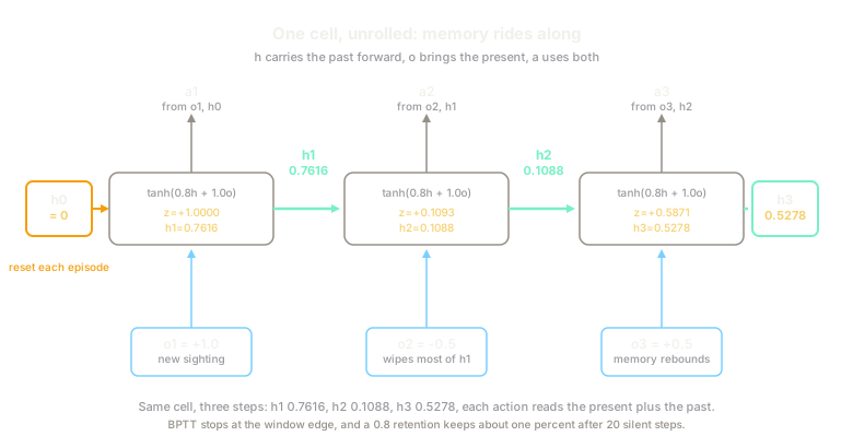
A tiny scalar cell, $h_{t+1} = \tanh(0.8\,h_t + 1.0\,o_t)$, starting from a reset $h_0 = 0$, watching observations $o = [+1.0, -0.5, +0.5]$:

• Step 0: $z_0 = 0.8 \times 0 + 1.0 \times 1.0 = 1.0000$. Then $h_1 = \tanh(1.0000) = 0.7616$. The strong positive sighting fills the memory.
• Step 1: $z_1 = 0.8 \times 0.7616 + 1.0 \times (-0.5) = 0.6093 - 0.5 = 0.1093$. Then $h_2 = \tanh(0.1093) = 0.1088$. The negative observation nearly wipes the slate, but $0.1088$ of history survives.
• Step 2: $z_2 = 0.8 \times 0.1088 + 1.0 \times 0.5 = 0.0870 + 0.5 = 0.5871$. Then $h_3 = \tanh(0.5871) = 0.5278$.

Notice step 1 and step 2 both faced middling inputs, yet the memory differs ($0.1088$ versus $0.5278$) because the past differs. That gap is the whole point: a feedforward net would treat similar frames identically, while this policy remembers. The diagram above draws exactly this unroll. And the vanishing side: after 20 silent steps the retention factor is $0.8^{20} = 0.0115$, barely one percent, which is why distant clues fade without gates.

Code

A standalone replay of the worked unroll, plus the decay check:

1import math2
3
4def unroll(observations: list[float], w_h: float = 0.8, w_x: float = 1.0) -> list[float]:5    """Run one scalar recurrent cell over an observation sequence.6
7    Returns the hidden state after each step, starting from a reset h = 0.8    """9    h = 0.010    states: list[float] = []11    for t, o in enumerate(observations):12        z = w_h * h + w_x * o13        h = math.tanh(z)14        print(f"step {t}: obs={o:+.1f} z={z:+.4f} h={h:+.4f}")15        states.append(h)16    return states17
18
19if __name__ == "__main__":20    unroll([1.0, -0.5, 0.5])21    print(f"decay over 20 steps: {0.8**20:.4f}")

1# -> expected output:2step 0: obs=+1.0 z=+1.0000 h=+0.76163step 1: obs=-0.5 z=+0.1093 h=+0.10884step 2: obs=+0.5 z=+0.5871 h=+0.52785decay over 20 steps: 0.0115

Watch Out For

The Quick Version

• A feedforward policy maps one observation to one action, so aliased views of different true states force identical moves. Partial observability is what breaks it.
• A recurrent policy carries a hidden state $h_t$ updated by $h_{t+1} = \tanh(W_h h_t + W_x o_t + b)$, and acts from both the observation and the memory.
• DRQN adds an LSTM to a Q-network and trains on sequences; recurrent PPO stores hidden states in its rollout buffer and replays short windows. Both reset memory at episode ends.
• BPTT trains through a truncated window, so dependencies longer than the window are unlearnable no matter how wide the hidden state is.
• Gated cells (LSTM, GRU) exist because plain recurrences fade: a retention of $0.8$ keeps only about one percent of a clue after 20 silent steps.

What to Read Next

• Deep Reinforcement Learning
• Deep Q-Networks
• Temporal Difference Learning
• Hierarchical RL