Deep Reinforcement Learning

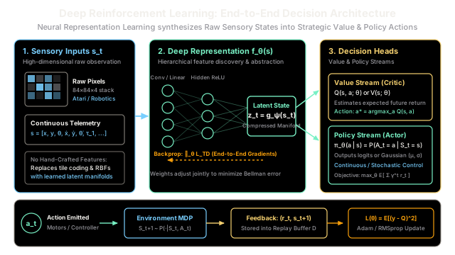
Why Does This Exist?

Classical reinforcement learning algorithms were developed on discrete, low-dimensional state spaces where an agent could store value estimates in a lookup table. However, tabular methods collapse under the curse of dimensionality. In an environment observed through an $84 \times 84$ 8-bit grayscale camera feed, the number of distinct raw pixel configurations is:

This vastly exceeds the estimated $10^{80}$ atoms in the observable universe. Lookup tables cannot represent this space, and an agent will almost never visit the exact same raw observation twice.

Early value function approximation attempted to solve this using linear models $\hat{v}(s, \mathbf{w}) = \mathbf{w}^\top \mathbf{x}(s)$, relying on hand-crafted basis functions such as polynomial bases, tile coding, and radial basis functions. While linear methods offer strong convergence guarantees, they shift the burden to human engineers who must manually invent feature extractors $\mathbf{x}(s)$. For unstructured high-dimensional observations—such as raw video frames, lidar point clouds, or continuous multi-joint torque sensors—manual feature engineering fails completely because human intuition cannot hand-tune representations that remain invariant to lighting changes, camera perspective shifts, and complex object interactions.

Deep Reinforcement Learning (Deep RL) solves this by replacing manual feature design with end-to-end representation learning. Deep neural networks automatically learn hierarchical feature abstractions directly from raw sensory observations: early layers detect edges and textures, intermediate layers capture spatial and temporal dynamics, and final decision heads output action values or policy distributions—all optimized simultaneously via reward feedback.

Think of It Like This

How It Actually Works

The Synthesis of Representation Learning and Sequential Decision Making

In a standard Markov Decision Process defined by the tuple $(\mathcal{S}, \mathcal{A}, \mathcal{P}, \mathcal{R}, \gamma)$, the state space $\mathcal{S}$ in Deep RL is high-dimensional: $\mathcal{S} \subset \mathbb{R}^d$ or $\mathcal{S} \subset \mathbb{R}^{H \times W \times C}$.

Instead of a linear model $\hat{v}(s, \mathbf{w}) = \mathbf{w}^\top \mathbf{x}(s)$, Deep RL parameterizes functions using a deep neural network with weights $\boldsymbol{\theta}$:

where:

• $g_{\boldsymbol{\psi}}: \mathcal{S} \to \mathbb{R}^k$ is an encoder network (such as convolutional or transformer layers) parameterized by weights $\boldsymbol{\psi}$ that projects high-dimensional observations into a compact latent representation $\mathbf{z} = g_{\boldsymbol{\psi}}(s)$.
• $h_{\boldsymbol{\phi}}: \mathbb{R}^k \to \mathbb{R}^{|\mathcal{A}|}$ is a decision head parameterized by weights $\boldsymbol{\phi}$ that maps the latent state $\mathbf{z}$ to value estimates or action probabilities.
• $\boldsymbol{\theta} = \{\boldsymbol{\psi}, \boldsymbol{\phi}\}$ represents all trainable network parameters optimized jointly end-to-end.

1+--------------------------------------------------------------------------------+2|                             DEEP RL TAXONOMY                                   |3+--------------------------------------------------------------------------------+4| 1. Value-Based       | Q_θ(s, a) ≈ Q*(s, a)      | DQN, Double DQN, Rainbow    |5| 2. Policy-Based      | π_θ(a | s) ≈ π*(a | s)    | REINFORCE, PPO, TRPO        |6| 3. Actor-Critic      | Actor π_θ + Critic Q_ϕ    | A2C, SAC, TD3               |7| 4. Model-Based       | T_ψ(z_t, a_t) → z_{t+1}   | World Models, MuZero, Dreamer|8+--------------------------------------------------------------------------------+

1. Value-Based Deep RL

Value-based methods parameterize the action-value function $Q_{\boldsymbol{\theta}}(s, a)$. The network parameters are updated by minimizing the Temporal Difference (TD) Mean Squared Bellman Error:

where $\mathcal{D}$ is an experience replay buffer and $\boldsymbol{\theta}^-$ represents periodic target network parameters held fixed to stabilize bootstrapping.

2. Policy-Based & Actor-Critic Deep RL

Policy-based methods parameterize a stochastic policy $\pi_{\boldsymbol{\theta}}(a \mid s)$ directly. The network parameters are optimized via gradient ascent on expected return $J(\boldsymbol{\theta}) = \mathbb{E}_{\tau \sim \pi_{\boldsymbol{\theta}}} [G_0]$:

where $A^{\pi}(s, a) = Q^{\pi}(s, a) - V^{\pi}(s)$ is the Advantage function, frequently estimated by a learned neural critic $V_{\boldsymbol{\phi}}(s)$.

The Four Core Theoretical Challenges of Deep RL

Training neural networks with reinforcement learning differs fundamentally from supervised learning due to four structural obstacles:

1. Non-Stationary Optimization Targets: In supervised learning, regression targets $y$ are fixed ground-truth labels. In Deep RL, the target $y = r + \gamma \max_{a'} Q_{\boldsymbol{\theta}}(s', a')$ depends on the very network weights $\boldsymbol{\theta}$ being updated, causing feedback loops and destabilization.
2. Correlated, Non-i.i.d. Data: Supervised learning assumes independent and identically distributed (i.i.d.) training samples. In RL, sequential exploration produces temporally autocorrelated trajectory streams ($s_{t+1}$ depends directly on $s_t$), which biases gradient updates.
3. Representation Collapse & Catastrophic Forgetting: As an agent moves between different regions of an environment, updates on new states overwrite latent representations learned for earlier states.
4. The Deadly Triad: Combining function approximation (neural networks), bootstrapping (TD learning), and off-policy sampling can cause value estimates to diverge to infinity.

Worked numerical example

Let us trace a single complete forward pass, Bellman target computation, and analytical backpropagation update for a 2-layer Neural Network Q-function.

1. Architecture and Initial Parameters

Consider an agent in a continuous 2D state space $\mathcal{S} \subset \mathbb{R}^2$ with two discrete actions $\mathcal{A} = \{0, 1\}$.

• Input state: $\mathbf{s} = \begin{bmatrix} 1.0 \\ 0.5 \end{bmatrix}$.
• Hidden layer (2 units, ReLU activation): $$\mathbf{W}_1 = \begin{bmatrix} 0.5 & -0.2 \\ 0.4 & 0.6 \end{bmatrix}, \quad \mathbf{b}_1 = \begin{bmatrix} 0.1 \\ -0.1 \end{bmatrix}$$
• Output layer (2 units, linear Q-values): $$\mathbf{W}_2 = \begin{bmatrix} 0.8 & -0.5 \\ 0.3 & 0.7 \end{bmatrix}, \quad \mathbf{b}_2 = \begin{bmatrix} 0.2 \\ -0.3 \end{bmatrix}$$
• Step size (learning rate): $\alpha = 0.1$.
• Discount factor: $\gamma = 0.90$.

2. Forward Pass

Compute the hidden layer pre-activations $\mathbf{z}_1$:

Applying the ReLU activation function $\mathbf{h} = \max(0, \mathbf{z}_1)$:

Compute the output layer action values $\mathbf{Q}(\mathbf{s}) = \mathbf{W}_2 \mathbf{h} + \mathbf{b}_2$:

The network predicts initial Q-values: $\mathbf{Q}(\mathbf{s}) = \begin{bmatrix} 0.30 \\ 0.27 \end{bmatrix}$.

3. Transition and Bellman Target

The agent executes action $a = 0$, receives scalar reward $r = 1.0$, and transitions to next state $\mathbf{s}'$. A separate target network evaluates $\mathbf{s}'$, yielding $\mathbf{Q}_{\text{target}}(\mathbf{s}') = \begin{bmatrix} 0.50 \\ 0.80 \end{bmatrix}$. The maximum target value is:

Compute the 1-step TD target $y$:

The TD error for chosen action $a = 0$ is:

The Mean Squared Error loss on action $0$ is:

4. Analytical Backpropagation

The output error gradient vector is non-zero only for the executed action $a = 0$:

Gradients for the second layer:

Backpropagate error to hidden pre-activations through ReLU:

Because both $z_{1, 1} = 0.50 > 0$ and $z_{1, 2} = 0.60 > 0$, the ReLU derivatives are $1.0$:

Gradients for the first layer:

5. Parameter Update

Applying gradient descent with step size $\alpha = 0.1$:

6. Verification with Updated Forward Pass

Re-evaluating state $\mathbf{s} = [1.0, 0.5]^\top$ with the updated parameters:

In a single gradient step, $Q(\mathbf{s}, 0)$ increased from $0.30$ to $0.8175$, closing $36.4\%$ of the initial error gap toward target $1.72$.

Code

The following self-contained Python script implements a pure NumPy 2-layer Deep Q-Network with forward propagation, Bellman target computation, analytical backpropagation, and training loop assertions.

1from typing import NamedTuple, Tuple2import numpy as np3
4
5class Transition(NamedTuple):6    state: np.ndarray7    action: int8    reward: float9    next_state: np.ndarray10    done: bool11
12
13class DeepQNetwork:14    """Two-layer MLP Q-network trained with analytical backpropagation."""15
16    def __init__(17        self,18        state_dim: int,19        hidden_dim: int,20        action_dim: int,21        lr: float = 0.08,22        seed: int = 42,23    ) -> None:24        self.lr = lr25        rng = np.random.default_rng(seed)26        # He initialization for ReLU activation27        self.W1 = rng.standard_normal((hidden_dim, state_dim)) * np.sqrt(28            2.0 / state_dim29        )30        self.b1 = np.zeros(hidden_dim)31        self.W2 = rng.standard_normal((action_dim, hidden_dim)) * np.sqrt(32            2.0 / hidden_dim33        )34        self.b2 = np.zeros(action_dim)35
36    def forward(37        self, state: np.ndarray38    ) -> Tuple[np.ndarray, np.ndarray, np.ndarray]:39        """Forward pass returning Q-values, hidden activations, and pre-activations."""40        z1 = self.W1 @ state + self.b141        h1 = np.maximum(0.0, z1)42        q_values = self.W2 @ h1 + self.b243        return q_values, h1, z144
45    def compute_td_target(46        self,47        reward: float,48        next_state: np.ndarray,49        done: bool,50        gamma: float = 0.90,51    ) -> float:52        """Compute 1-step Bellman target."""53        if done:54            return float(reward)55        next_q, _, _ = self.forward(next_state)56        return float(reward + gamma * np.max(next_q))57
58    def update(59        self, state: np.ndarray, action: int, target: float60    ) -> Tuple[float, float]:61        """Perform analytical backpropagation step for a single transition."""62        q_vals, h1, z1 = self.forward(state)63        pred_q = q_vals[action]64        td_error = target - pred_q65        loss = 0.5 * (td_error**2)66
67        # Output layer gradient68        grad_out = np.zeros_like(q_vals)69        grad_out[action] = pred_q - target70
71        grad_W2 = np.outer(grad_out, h1)72        grad_b2 = grad_out.copy()73
74        # Hidden layer backpropagation75        grad_h1 = self.W2.T @ grad_out76        grad_z1 = grad_h1 * (z1 > 0.0)  # ReLU derivative77        grad_W1 = np.outer(grad_z1, state)78        grad_b1 = grad_z1.copy()79
80        # Gradient descent parameter updates81        self.W2 -= self.lr * grad_W282        self.b2 -= self.lr * grad_b283        self.W1 -= self.lr * grad_W184        self.b1 -= self.lr * grad_b185
86        return float(loss), float(td_error)87
88
89if __name__ == "__main__":90    q_net = DeepQNetwork(91        state_dim=2, hidden_dim=4, action_dim=2, lr=0.08, seed=4292    )93
94    # Sample batch of transitions from a continuous 2D environment95    dataset = [96        Transition(97            state=np.array([1.0, 0.5]),98            action=0,99            reward=1.0,100            next_state=np.array([0.8, 0.2]),101            done=False,102        ),103        Transition(104            state=np.array([-0.5, 1.2]),105            action=1,106            reward=-0.5,107            next_state=np.array([-0.2, 0.9]),108            done=False,109        ),110        Transition(111            state=np.array([0.3, -0.8]),112            action=0,113            reward=2.0,114            next_state=np.array([0.0, 0.0]),115            done=True,116        ),117    ]118
119    print("=== Initial Q-Predictions ===")120    for i, t in enumerate(dataset):121        q, _, _ = q_net.forward(t.state)122        print(f"State {i}: Q(s, 0) = {q[0]:.4f}, Q(s, 1) = {q[1]:.4f}")123
124    # Mini-batch training loop125    for epoch in range(1, 101):126        total_loss = 0.0127        for t in dataset:128            target = q_net.compute_td_target(129                t.reward, t.next_state, t.done, gamma=0.90130            )131            loss, _ = q_net.update(t.state, t.action, target)132            total_loss += loss133        if epoch in [1, 25, 50, 100]:134            print(f"Epoch {epoch:3d} | Total TD Loss: {total_loss:.6f}")135
136    print("\n=== Converged Q-Predictions ===")137    for i, t in enumerate(dataset):138        q, _, _ = q_net.forward(t.state)139        best_act = int(np.argmax(q))140        print(141            f"State {i}: Q(s, 0) = {q[0]:.4f}, Q(s, 1) = {q[1]:.4f} -> Greedy Action: {best_act}"142        )143
144    # Verification assertions145    assert (146        total_loss < 0.01147    ), f"Expected converged loss < 0.01, got {total_loss}"148    final_q0, _, _ = q_net.forward(dataset[0].state)149    assert final_q0[0] > 3.0, f"Expected Q(s0, 0) > 3.0, got {final_q0[0]}"150    print("\nAll assertions passed successfully!")151
152# Expected Output:153# === Initial Q-Predictions ===154# State 0: Q(s, 0) = -0.7363, Q(s, 1) = 0.9730155# State 1: Q(s, 0) = -0.4545, Q(s, 1) = 0.6006156# State 2: Q(s, 0) = 0.4331, Q(s, 1) = 0.0170157# Epoch   1 | Total TD Loss: 3.744165158# Epoch  25 | Total TD Loss: 0.011526159# Epoch  50 | Total TD Loss: 0.000000160# Epoch 100 | Total TD Loss: 0.000000161#162# === Converged Q-Predictions ===163# State 0: Q(s, 0) = 4.1507, Q(s, 1) = 0.7383 -> Greedy Action: 0164# State 1: Q(s, 0) = 2.1358, Q(s, 1) = 1.6480 -> Greedy Action: 0165# State 2: Q(s, 0) = 2.0000, Q(s, 1) = 0.0300 -> Greedy Action: 0166#167# All assertions passed successfully!

Watch Out For

The Quick Version

• End-to-End Perception: Deep RL replaces hand-engineered feature representations (tile coding, radial basis functions) with deep neural networks that learn spatial and temporal abstractions directly from raw sensory inputs.
• The Core Architecture: High-dimensional observations pass through an encoder network into a latent representation $\mathbf{z} = g_{\boldsymbol{\psi}}(s)$, which branches into decision heads predicting value functions $Q(s, a)$ or parameterized policies $\pi(a \mid s)$.
• Optimization Challenges: Unlike supervised learning, Deep RL optimizes against moving, self-referential Bellman targets over non-i.i.d., temporally correlated trajectories, rendering training vulnerable to divergence and representation collapse.
• Stabilization Mechanisms: Practical Deep RL algorithms rely on experience replay buffers, Polyak target networks, clipped objectives (PPO), and actor-critic architectures to tame optimization instability.

What to Read Next

• Deep Q-Networks
• Experience Replay
• Policy Gradient Methods
• Advanced and PhD-Level Topics in RL