Regret Bounds

Regret is the gap between the reward you got and the reward perfect play would have earned. Good learners make that gap grow slower than time itself.

Cumulative regret from a 10-pull two-arm trace stays at 0.9 while the square-root envelope bends below the linear never-learn line.

Why Does This Exist?

Total reward alone cannot tell you whether an agent is learning. A slot machine that pays 0.4 per pull looks fine until you learn the machine next to it pays 0.7. The missing piece is the gap to perfect play, added up over time. That gap is regret, and a regret bound is a promise about how fast the gap grows.

This matters because exploration has a bill. Every pull of a worse arm, every episode with a shaky policy, pays it. Without a bound you cannot say whether multi-armed bandits algorithm A beats algorithm B, or whether your agent is improving or just lucky. With one, you get a number you can plot: linear means the agent never learns, sublinear means its average shortfall shrinks toward zero.

This page covers the definition, the two classic growth rates, and the optimism idea that earns them. Your prerequisites are the bandit setup and the upper confidence bound rule, plus the exploration versus exploitation tradeoff for motivation. The bandit page introduces regret in passing; the UCB page proves the bandit rate. Here you get the full picture and the lift from bandits to MDPs.

Think of It Like This

The new office lunch counters

You join an office with two lunch counters. Counter Best serves a meal worth 7 points to you. Counter Meh serves one worth 4 points. You do not know the scores yet, so you try both for ten days.

Each Meh day costs you 3 points of tastiness you could have had. That daily shortfall is instantaneous regret. Add it over ten days with three Meh visits and your cumulative regret is 9 points. The curve in the diagram is your lunch diary: it jumps by 3 on Meh days and stays flat on Best days.

A friend who never learns keeps picking at random and their diary climbs like a staircase forever. You learn: after day 6 you stop visiting Meh, your curve goes flat, and your average regret per day falls from 0.3 toward zero.

Where the analogy stops: lunch scores stay fixed and one meal never affects the next. In an MDP, today's action changes tomorrow's state, so regret has to compare whole policies from a start state, not single pulls. Delayed consequences make the bound carry extra factors for horizon, states, and actions.

How It Actually Works

The definition: cumulative regret

Fix $K$ episodes (or rounds), indexed by $k = 1$ to $K$ . Let $V^{\star}$ be the value of the optimal policy from the start state, meaning the best long-term return anyone could get. Let $V^{\pi_{k}}$ be the value of the policy the agent actually used in episode $k$ . Then cumulative regret is:

$\mathrm{Regret}(K) = \sum_{k=1}^{K} \left( V^{\star} - V^{\pi_{k}} \right)$

Every symbol in plain words: $K$ counts how long you played, $V^{\star}$ is perfect play's score, $\pi_{k}$ is what you did in episode $k$ , and each bracket term is what you left on the table that episode. In a bandit there is no state, so $V^{\star}$ is the best arm's mean $\mu^{\star}$ and $V^{\pi_{k}}$ is the chosen arm's mean. The formula is the same shape, only simpler.

The headline test: regret is sublinear when $\mathrm{Regret}(K) / K$ shrinks toward zero as $K$ grows. Put plainly, your average mistake per episode vanishes. Linear regret, say $0.3K$ , means you keep making the same mistake forever and never catch up.

Logarithmic versus square-root regret

Two regimes show up everywhere, and mixing them up causes real confusion.

Gap-dependent (logarithmic) bounds apply when the smallest gap $\Delta$ between the best and second-best option stays fixed above zero. Then a good algorithm needs only about $\log K / \Delta^{2}$ pulls of each worse arm, and expected regret grows like $\log K / \Delta$ . The $\log K$ grows so slowly it looks almost flat: $\ln(10) \approx 2.30$ , $\ln(1000) \approx 6.91$ , $\ln(1000000) \approx 13.82$ . I computed those three values directly. At a million episodes the log term is still under 14 while $\sqrt{1000000} = 1000$ . When gaps are fixed, logarithmic regret wins by a mile.

Gap-independent (square-root) bounds hold even when $\Delta$ can be tiny or shrink with $K$ . Then the worst-case price is on the order of $\sqrt{K}$ up to log factors. No algorithm beats that in general: when two arms differ by $1 / \sqrt{K}$ , telling them apart takes about $K$ pulls, so $\sqrt{K}$ regret is unavoidable. Think of it as two promises. The log bound says life is cheap when answers are clear. The sqrt bound says learning still works when answers are murky, at a steeper but still sublinear price.

Our worked trace sits far under both at $K = 10$ , which is normal. Bounds describe growth, not tight small- $K$ predictions. The log bound's constants are loose early and the sqrt envelope sits high early; the payoff appears as $K$ grows and the curves bend while linear regret keeps climbing.

How optimism earns the bound

The engine behind both rates is optimism in the face of uncertainty. Keep a confidence interval around every estimate, then act as if the most favorable plausible world were true.

In bandits the upper confidence bound rule picks the arm maximizing sample mean plus bonus:

$A_{k} = \arg\max_{a} \left[ Q_{k}(a) + c \sqrt{\frac{\ln k}{N_{k}(a)}} \right]$

Here $Q_{k}(a)$ is the average reward seen from arm $a$ so far, $N_{k}(a)$ counts its pulls, $k$ is the round, and $c$ sets confidence width. The bonus shrinks each time you pull an arm and grows slowly with $k$ for arms you neglect, so no arm starves. A standard concentration argument shows each worse arm is pulled only $O(\log K / \Delta^{2})$ times, and multiplying pulls by per-pull cost $\Delta$ gives $O(\log K / \Delta)$ regret. Shrink $\Delta$ toward zero and the same argument degrades gracefully to the $\sqrt{K}$ rate.

The lift to MDPs keeps the same skeleton and pays for dynamics. Instead of one bonus per arm, optimistic algorithms keep confidence sets over rewards and transitions for each state-action pair, plan as if the best plausible model were true, act, then shrink the sets with fresh data. Early tabular versions do this with extended value iteration over the confidence set; later ones add an exploration bonus straight into the Bellman backup, roughly proportional to $1 / \sqrt{N(s, a)}$ where $N(s, a)$ counts visits. The value estimates inside those backups are the same bootstrapped quantities temporal-difference learning computes, now with a bonus glued on. Regret keeps its definition, $\sum_{k}(V^{\star} - V^{\pi_{k}})$ , and the bound picks up the MDP size, growing with horizon, states, and actions under the square root plus log factors. That is the bandit-to-MDP lift: same optimism, wider uncertainty, heavier but still sublinear bill.

Worked 2-arm trace: gap 0.3 over 10 episodes

Two arms. Best pays mean $\mu^{\star} = 0.7$ , the other pays $0.4$ , so the gap is $\Delta = 0.7 - 0.4 = 0.3$ . Play $K = 10$ episodes with this fixed pull order, writing 1 for a miss and 0 for the best arm:

$[1, 0, 1, 0, 0, 1, 0, 0, 0, 0]$

Instantaneous expected regret is $0.3$ on a 1 and $0$ on a 0. Accumulate it:

Episode 1 (miss): $0.3$ , cumulative $0.3$ .
Episode 2 (best): adds $0$ , cumulative stays $0.3$ .
Episode 3 (miss): adds $0.3$ , cumulative $0.6$ .
Episodes 4 to 5 (best, best): cumulative stays $0.6$ .
Episode 6 (miss): adds $0.3$ , cumulative $0.9$ .
Episodes 7 to 10 (best each time): cumulative stays $0.9$ .

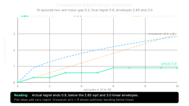
Full trace: $[0.3, 0.3, 0.6, 0.6, 0.6, 0.9, 0.9, 0.9, 0.9, 0.9]$ . Final regret $0.9$ , average regret $0.09$ per episode. I computed every entry by hand and confirmed it with the script in the Code section.

Now compare against the two reference lines in the diagram, both computed for the same $K$ . The never-learn line pulls the worse arm every round: $0.3K$ , which is $3.0$ at $K = 10$ . The drawn square-root envelope is $0.9\sqrt{k}$ , which is about $2.85$ at $K = 10$ since $\sqrt{10} \approx 3.16$ . Our trace ends at $0.9$ , under both. The two references cross exactly at $k = 9$ , where $0.9 \times 3 = 2.7$ equals $0.3 \times 9 = 2.7$ . Before the crossing the sqrt curve rides higher; after it, the sqrt curve bends below the straight line. That bend is the whole visual argument: sublinear growth flattens while linear growth never does.

Code

This short script replays the exact trace above. Pull code 1 means the worse arm, 0 means the best arm. Run it and check the printed trace against the diagram's stepped line.

1from typing import List2
3
4def cumulative_regret(pulls: List[int], mu_star: float, mu_sub: float) -> List[float]:5    """Expected cumulative regret for a fixed pull order."""6    gap = mu_star - mu_sub7    total = 0.08    trace: List[float] = []9    for a in pulls:10        if a == 1:11            total += gap12        trace.append(round(total, 2))13    return trace14
15
16pulls = [1, 0, 1, 0, 0, 1, 0, 0, 0, 0]17trace = cumulative_regret(pulls, 0.7, 0.4)18print(trace)19print("final:", trace[-1], "average:", round(trace[-1] / len(trace), 4))

1# -> expected output:2[0.3, 0.3, 0.6, 0.6, 0.6, 0.9, 0.9, 0.9, 0.9, 0.9]3final: 0.9 average: 0.09

Watch Out For

Sublinear is not zero regret

A flat-looking curve can still hide a big bill. Our trace ends at 0.9 after 10 episodes, which is 0.09 per episode of missed value. Sublinear only promises the per-episode average keeps shrinking as episodes grow, not that early regret was small. The fix: always quote regret with its horizon. Say 0.9 after 10 episodes and report the average 0.09 alongside it. Never compare one paper's 900 against another's 90 when their horizons differ by a factor of 100.

The horizon and the MDP size ride along

Bandit intuition understates MDP regret. Each extra horizon step, state, or action widens the confidence sets, so the same bonus that explores a 2-arm bandit in 10 pulls can take orders of magnitude longer in a long-horizon MDP. Symptom: a bonus tuned on bandits stalls in gridworlds because rarely visited state-action pairs stay overconfident. The fix: keep the horizon fixed when comparing curves, normalize regret per episode, and expect the bound to grow with horizon, states, and actions under the root rather than staying a pure function of episode count.

The Quick Version

Cumulative regret is the total shortfall to perfect play: the sum over episodes of optimal value minus the value of the policy actually used.
Regret is sublinear when average regret per episode shrinks toward zero, which is the precise meaning of an agent that keeps learning.
A fixed gap between best and rest gives logarithmic regret like UCB achieves in bandits, while tiny or shrinking gaps cost square-root regret in the worst case.
Optimism earns both rates by acting on the best plausible estimates and shrinking confidence intervals with each visit, from bandit bonuses to MDP-wide optimistic planning.
Our 2-arm trace with gap 0.3 and three misses in 10 episodes ends at regret 0.9, sitting below the 2.85 square-root envelope and the 3.0 never-learn line.