Risk-Sensitive RL

Risk-sensitive RL picks policies by the shape of their return distribution, not just the average, so a steady policy can beat a flashy gamble with the same mean.

Two policies share mean return 10, but the narrow distribution has CVaR 8 while the wide one has CVaR minus 10, so a risk-averse objective picks the steady policy.

Why Does This Exist?

Standard reinforcement learning maximizes expected return. The agent learns the action with the highest average outcome $Q(s, a) = \mathbb{E}[Z(s, a)]$ , where $Z(s, a)$ is the full distribution over future returns and $Q(s, a)$ is just its mean. That works when every bad outcome is cheap and reversible. It breaks the moment a rare catastrophe matters more than a slightly better average: a trading bot that earns a little extra most days but wipes out the account one day in twenty, or a delivery robot that is fast on average but occasionally drives down stairs.

The mean erases that difference. Two policies can share exactly the same expected return while one of them fails catastrophically 25% of the time. A risk-neutral agent cannot tell them apart, so it may happily deploy the dangerous one.

This page covers the fix: objectives that score a policy by the shape of its return distribution. You will see variance penalties, quantile objectives, and CVaR (conditional value at risk), plus what it means to be risk-averse versus risk-seeking. It doesn't re-teach how those distributions get learned. That machinery lives on the neighbour pages: QR-DQN learns return quantiles directly, and C51 learns a categorical return distribution. When risk means hard constraints rather than preferences, that is safe RL.

Think of It Like This

Two commutes with the same average

You have two routes to work. Route A takes 30 minutes every single day. Route B takes 15 minutes nine days out of ten, but 165 minutes on the tenth day when the bridge jams. Check the average: $0.9 \times 15 + 0.1 \times 165 = 13.5 + 16.5 = 30$ minutes. Same average, very different experience.

On interview day you take route A without thinking. You are being risk-averse: you care about the worst case, not the average. On a lazy Saturday with nowhere to be, you might take route B for the thrill of the fast run. That's risk-seeking: you care about the upside. Same roads, same average, opposite choice, because your objective changed.

Where the analogy stops: you can see commute times directly, but an RL agent must estimate its return distribution from samples. Rare tails are the hardest part to estimate, because by definition few samples land there. Keep that in mind when you read the second pitfall below.

How It Actually Works

From expected return to risk measures

Write the return of a policy $\pi$ as a random variable $Z^\pi$ . Risk-neutral RL maximizes its mean:

$J_{\text{neutral}}(\pi) = \mathbb{E}[Z^\pi]$

Risk-sensitive RL replaces the mean with a functional that reacts to spread and tails. Three workhorses:

Variance penalty. $J(\pi) = \mathbb{E}[Z^\pi] - \lambda \, \mathrm{Var}(Z^\pi)$ , with $\lambda > 0$ setting how much spread you punish. Here $\mathrm{Var}$ is the variance (squared spread around the mean) and $\lambda$ (lambda) is your price per unit of variance. Simple, differentiable, but it punishes upside surprises exactly as much as disasters.
Quantile objective. Pick a level $\tau$ (tau) between 0 and 1 and maximize the $\tau$ -quantile $q_\tau$ , the return value that the policy beats with probability $1 - \tau$ . A low quantile ( $q_{0.1}$ , the value beaten 90% of the time) is a pessimistic, risk-averse target. A high quantile ( $q_{0.9}$ ) is optimistic and risk-seeking: it chases the best case.
CVaR objective. $\text{CVaR}_\alpha$ (conditional value at risk at level $\alpha$ , alpha) is the average return over the worst $\alpha$ fraction of outcomes. $\text{CVaR}_{0.25}$ is the mean of the worst quarter. Maximizing it means maximizing the floor, not the average. This is the favorite of practitioners who answer for worst cases.

None of this requires new learning machinery. If you already have return quantiles from QR-DQN, CVaR is just the average of the bottom quantiles, and a quantile objective is just one entry of the vector. Risk sensitivity is a choice of what to optimize, layered on top of the distributional view.

Risk-averse means $\lambda > 0$ , low quantiles, or CVaR: you sacrifice average performance to lift the floor. Risk-seeking flips the sign: you accept a worse average for a shot at the ceiling, which is sometimes exactly right, for example when only the single best trajectory in a research sweep gets published.

Worked example: same mean, opposite ranking

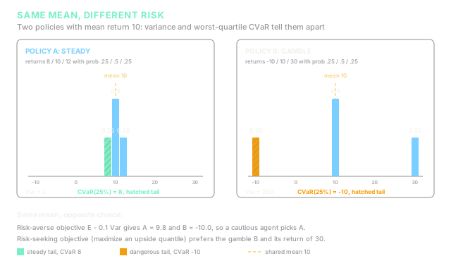
Two policies, each with three possible episode returns. Policy A is steady; policy B gambles.

Policy A: return 8 with probability 0.25, 10 with probability 0.5, 12 with probability 0.25.

$\mathbb{E}[Z_A] = 0.25 \times 8 + 0.5 \times 10 + 0.25 \times 12 = 2 + 5 + 3 = 10$

$\mathbb{E}[Z_A^2] = 0.25 \times 64 + 0.5 \times 100 + 0.25 \times 144 = 16 + 50 + 36 = 102$

$\mathrm{Var}(Z_A) = 102 - 10^2 = 2$

Policy B: return $-10$ with probability 0.25, 10 with probability 0.5, 30 with probability 0.25.

$\mathbb{E}[Z_B] = 0.25 \times (-10) + 0.5 \times 10 + 0.25 \times 30 = -2.5 + 5 + 7.5 = 10$

$\mathbb{E}[Z_B^2] = 0.25 \times 100 + 0.5 \times 100 + 0.25 \times 900 = 25 + 50 + 225 = 300$

$\mathrm{Var}(Z_B) = 300 - 10^2 = 200$

Same mean (10), but B's variance is one hundred times A's. Now the tail view. The worst quarter of episodes is exactly the bottom atom in each case (probability 0.25), so:

$\text{CVaR}_{0.25}(A) = 8, \qquad \text{CVaR}_{0.25}(B) = -10$

And the variance-penalized objective with $\lambda = 0.1$ :

$J(A) = 10 - 0.1 \times 2 = 9.8, \qquad J(B) = 10 - 0.1 \times 200 = -10.0$

A risk-neutral agent ties them at 10 to 10. A risk-averse agent ( $\lambda = 0.1$ , or CVaR) picks A by a landslide. A risk-seeking agent maximizing the 0.9-quantile picks B, since B's top quarter returns 30 against A's 12. The diagram at the top draws exactly these two distributions on one shared axis so you can see the shared mean and the different tails.

Code

Short script that scores both policies on mean, variance, CVaR at 25%, and the variance-penalized objective:

1def cvar(outcomes: list[tuple[float, float]], alpha: float = 0.25) -> float:2    """Mean return over the worst alpha fraction of episodes."""3    need, total = alpha, 0.04    for x, p in sorted(outcomes):5        take = min(p, need)6        total += take * x7        need -= take8        if need <= 0:9            break10    return total / alpha11
12
13def score(outcomes: list[tuple[float, float]], lam: float = 0.1) -> dict[str, float]:14    """Score a discrete return distribution given as (value, prob) pairs."""15    mean = sum(x * p for x, p in outcomes)16    var = sum(p * (x - mean) ** 2 for x, p in outcomes)17    penalized = mean - lam * var18    return {"mean": mean, "var": var, "cvar25": cvar(outcomes), "penalized": penalized}19
20
21steady = [(8.0, 0.25), (10.0, 0.5), (12.0, 0.25)]22gamble = [(-10.0, 0.25), (10.0, 0.5), (30.0, 0.25)]23
24for name, policy in [("steady", steady), ("gamble", gamble)]:25    print(name, score(policy))

1# -> expected output:2steady {'mean': 10.0, 'var': 2.0, 'cvar25': 8.0, 'penalized': 9.8}3gamble {'mean': 10.0, 'var': 200.0, 'cvar25': -10.0, 'penalized': -10.0}

Watch Out For

Evaluating on the mean and deploying the gamble

You train two checkpoints, evaluate each over 50 episodes, and both average about 10. You ship the one with the slightly higher mean and learn in production that its tail contains account-wiping episodes yours never had. The symptom is a deploy that looks identical in the eval dashboard but behaves nothing like the incumbent on bad days.

Fix it by reporting the tail next to the mean: variance and $\text{CVaR}_{0.25}$ over the same eval episodes, computed by the snippet above. Select checkpoints on the risk objective you actually care about, not on the mean you happened to log.

Trusting a tail estimated from a handful of episodes

$\text{CVaR}_{0.05}$ estimated from 100 eval episodes rests on 5 episodes. One lucky run flips which policy looks safer, and the ranking reverses on the next eval. The symptom is a risk ranking that will not replicate: A beats B on Monday, B beats A on Tuesday, with identical code.

Fix it with more episodes, wider error bars, or a coarser level. Prefer $\text{CVaR}_{0.25}$ over $\text{CVaR}_{0.05}$ when eval budgets are small, and report a confidence interval around the tail estimate. A tail number without a sample count attached is a rumor, not a measurement.

The Quick Version

Standard RL maximizes the mean return, which cannot distinguish a steady policy from a gamble with the same average.
Risk-sensitive RL scores the whole return distribution instead, using variance penalties, quantile objectives, or CVaR (the average of the worst outcomes).
In the worked example both policies average 10, but variances are 2 versus 200 and $\text{CVaR}_{0.25}$ values are 8 versus $-10$ .
A variance penalty with $\lambda = 0.1$ scores the steady policy at 9.8 and the gamble at $-10.0$ , flipping a tie into a clear choice.
Risk-averse means lifting the floor (low quantiles, CVaR); risk-seeking means chasing the ceiling (high quantiles), which suits settings where only the best run counts.
Report tails next to means at eval time, and never trust a tail estimate built on a handful of episodes.