Soft Q-Learning

Soft Q-Learning augments standard Q-learning with an entropy bonus, replacing the rigid max operator with a smooth log-sum-exp soft value function that learns multimodal energy-based policies.

Why Does This Exist?

In classical reinforcement learning, value-based methods such as Deep Q-Networks (DQN) rely on the hard maximization operator to compute target values: $y = r + \gamma \max_{a'} Q(s', a')$ . While mathematically sound under exact tabular representations, this hard maximization introduces severe failure modes when applied to complex or continuous environments with function approximation:

Overestimation Bias and Maximization Noise: Evaluating a greedy $\max$ over noisy neural network estimates systematically overestimates action values due to Jensen's inequality. Even with target networks, small positive estimation errors compound across backup steps.
Premature Mode Collapse: Standard Q-learning forces the derived policy to collapse into a single deterministic action mode (the greedy $\arg\max_a Q(s, a)$ ). When an environment contains multiple equally viable solutions—such as steering left or right around an obstacle—greedy Q-learning prematurely picks one and completely discards the other. If an environmental shift suddenly blocks that chosen corridor, the agent cannot quickly pivot because it never learned alternative paths.
Exploration Freezes in Complex Landscapes: In high-dimensional tasks like robotic locomotion and dextrous manipulation, rewarding purely deterministic trajectories causes policies to get trapped in narrow, sub-optimal local basins.

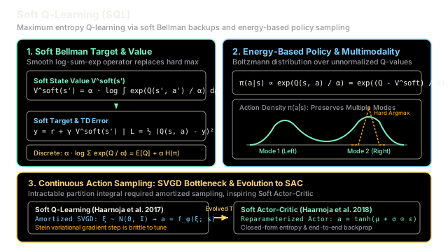
Soft Q-Learning (SQL), introduced by Haarnoja et al. in 2017, resolves these issues by reformulating Q-learning through the Maximum Entropy RL framework. Instead of training a policy to choose a single highest-value action, SQL trains an energy-based policy whose action density is proportional to exponentiated Q-values. By replacing the brittle hard $\max$ with a smooth, thermodynamically inspired log-sum-exp soft value function, SQL preserves multiple action modes, mitigates overestimation, and establishes the theoretical bridge between value iteration and modern actor-critic methods.

Think of It Like This

A Reservoir Filling Connected Valleys

Imagine water flowing into an uneven mountain basin composed of several distinct ravines and canyons of varying depths.

Traditional hard Q-learning behaves like an aggressive trench-digger. The moment it detects that one canyon floor is even a millimeter deeper than the others, it excavates a trench that redirects 100% of the water exclusively into that single sinkhole. Every other canyon is left bone-dry. If an unexpected boulder later falls into that single ravine, the entire water system becomes hopelessly blocked because no other channels were maintained.

Soft Q-Learning behaves like a rising natural reservoir governed by water temperature. The water level rises and pools across all connected depressions simultaneously. The deepest ravine naturally holds the highest volume of water, but secondary canyons also hold substantial pools proportional to their depth. Connecting passes remain submerged and accessible.

If conditions shift or a primary path is blocked, the reservoir is already flowing through the secondary channels without missing a beat. If the temperature $\alpha$ is gradually lowered, the water gently concentrates into the deepest depression; but while warm, the system maintains a presence in every viable basin.

Where the analogy stops: Physical water settles according to static terrain and gravity. In Soft Q-Learning, the "terrain" is an evolving neural network landscape $Q_\theta(s, a)$ continuously reshaped by Bellman errors, and the agent samples actions from an unnormalized energy distribution rather than a physical fluid.

How It Actually Works

Maximum Entropy RL and the Soft Bellman Equation

Standard reinforcement learning optimizes the cumulative expected discounted return $\sum_t \mathbb{E}[r(s_t, a_t)]$ . Soft Q-Learning augments this objective with policy entropy:

J(\pi) = \sum_{t=0}^\infty \mathbb{E}_{(s_t, a_t) \sim \rho_\pi} \left[ r(s_t, a_t) + \alpha \mathcal{H}(\pi(\cdot | s_t)) \right]

where:

$\mathcal{H}(\pi(\cdot | s_t)) = \mathbb{E}_{a \sim \pi}[-\log \pi(a | s_t)]$ represents the Shannon entropy of the policy at state $s_t$ .
$\alpha > 0$ is the entropy temperature hyperparameter controlling the trade-off between maximizing rewards and maintaining randomness.

Under this entropy-augmented objective, the optimal policy $\pi^*$ takes the form of an energy-based Boltzmann (Gibbs) distribution where unnormalized Q-values act as negative energies:

\pi^*(a | s) = \frac{\exp\left( \frac{Q^*(s, a)}{\alpha} \right)}{\int_{\mathcal{A}} \exp\left( \frac{Q^*(s, a')}{\alpha} \right) da'} = \exp\left( \frac{Q^*(s, a) - V^{\text{soft}}(s)}{\alpha} \right)

Substituting this energy-based optimal policy back into the soft state-value definition $V^{\text{soft}}(s) = \mathbb{E}_{a \sim \pi^*}[Q^*(s, a) - \alpha \log \pi^*(a | s)]$ yields the closed-form Soft Value Function:

V^{\text{soft}}(s) = \alpha \log \int_{\mathcal{A}} \exp\left( \frac{Q(s, a')}{\alpha} \right) da'

For discrete action spaces with $K$ actions $\{a_1, \dots, a_K\}$ , this integral simplifies to the smooth Log-Sum-Exp (LSE) operator:

V^{\text{soft}}(s) = \alpha \log \sum_{i=1}^K \exp\left( \frac{Q(s, a_i)}{\alpha} \right)

This soft value function possesses crucial mathematical properties:

Smoothness and Limit Behavior: As the temperature $\alpha \to 0$ , $V^{\text{soft}}(s) \to \max_a Q(s, a)$ , recovering standard hard Q-learning. As $\alpha \to \infty$ , the policy approaches a uniform random distribution, and $V^{\text{soft}}(s)$ approaches an average value plus maximal entropy.
Contraction Mapping: The soft Bellman operator $\mathcal{T}^{\text{soft}} Q(s, a) \triangleq r(s, a) + \gamma V^{\text{soft}}(s')$ is a contraction mapping in the supremum norm, guaranteeing convergence to a unique optimal soft Q-function $Q^*$ .

The neural network parameters $\theta$ are trained by minimizing the mean squared soft Bellman error over transitions sampled from an experience replay buffer $\mathcal{D}$ :

L(\theta) = \mathbb{E}_{(s, a, r, s') \sim \mathcal{D}} \left[ \frac{1}{2} \left( Q_\theta(s, a) - y^{\text{soft}} \right)^2 \right]

where the soft Bellman target $y^{\text{soft}}$ is evaluated using a slowly updated target network with parameters $\bar{\theta}$ :

y^{\text{soft}} = r + \gamma V_{\bar{\theta}}^{\text{soft}}(s') = r + \gamma \left( \alpha \log \int_{\mathcal{A}} \exp\left( \frac{Q_{\bar{\theta}}(s', a')}{\alpha} \right) da' \right)

Energy-Based Policies and Continuous Action Sampling via SVGD

In discrete action domains, executing the soft policy is straightforward: compute $Q(s, a_i)$ for all actions, evaluate the softmax probabilities $\pi(a_i | s) = \frac{\exp(Q(s, a_i)/\alpha)}{\sum_j \exp(Q(s, a_j)/\alpha)}$ , and sample a discrete action.

In continuous action spaces $\mathcal{A} \subseteq \mathbb{R}^d$ , however, two critical challenges emerge:

Intractable Target Integral: The partition integral $\int_{\mathcal{A}} \exp(Q(s, a')/\alpha) da'$ cannot be evaluated in closed form. SQL approximates it using importance sampling over $M$ action candidates drawn from a proposal distribution $q$ : $V^{\text{soft}}(s') \approx \alpha \log \left( \frac{1}{M} \sum_{j=1}^M \frac{\exp\left( Q(s', a^{(j)}) / \alpha \right)}{q(a^{(j)} | s')} \right)$
Action Sampling Bottleneck: The policy $\pi(a | s) \propto \exp(Q(s, a) / \alpha)$ is an unnormalized energy-based density. Simple Gaussian sampling cannot generate samples from arbitrary multimodal energy landscapes.

To sample actions efficiently, Haarnoja et al. (2017) trained an amortized deep sampling network $f_\phi(\xi; s)$ that transforms standard Gaussian noise $\xi \sim \mathcal{N}(0, I)$ into action samples $a = f_\phi(\xi; s)$ .

The sampler parameters $\phi$ are optimized using Stein Variational Gradient Descent (SVGD), which minimizes the Kullback-Leibler (KL) divergence between the sampler distribution $q_\phi$ and the target Boltzmann energy distribution $p(a|s) \propto \exp(Q(s, a)/\alpha)$ . The SVGD update on a set of action particles $\{a_i\}_{i=1}^N$ combines two opposing forces:

\Delta a_i \propto \frac{1}{N} \sum_{j=1}^N \left[ k(a_j, a_i) \nabla_{a_j} Q(s, a_j) + \alpha \nabla_{a_j} k(a_j, a_i) \right]

where $k(\cdot, \cdot)$ is a positive-definite Radial Basis Function (RBF) kernel. The first term acts as an attraction force, driving action particles uphill toward high Q-value regions. The second term acts as a repulsion force, preventing particles from collapsing onto the same mode and enforcing diverse, multimodal coverage across distinct peaks.

The Evolution from Soft Q-Learning to Soft Actor-Critic (SAC):
While Soft Q-Learning demonstrated unprecedented multimodal behavior in continuous robotic manipulation (such as learning multiple obstacle-avoidance maneuvers simultaneously), training the sampling network with SVGD was brittle, required carefully tuned kernel bandwidths, and imposed substantial computational overhead. In 2018, the authors introduced Soft Actor-Critic (SAC), which replaced the amortized SVGD sampler with a reparameterized Gaussian actor, achieving stable, end-to-end backpropagation while preserving the maximum entropy foundation.

Worked numerical example

Let us trace a single soft Bellman target update step on a discrete action space $\mathcal{A} = \{a_1, a_2\}$ :

Hyperparameters:
- Entropy temperature: $\alpha = 2.0$
- Discount factor: $\gamma = 0.9$
- Transition tuple: $(s, a, r = 1.5, s')$
- Current value estimate: $Q(s, a) = 5.0$
- Next-state target Q-values: $Q(s', a_1) = 4.0$ and $Q(s', a_2) = 2.0$

Step 1: Compute scaled logits and partition sum Scale the target Q-values by the temperature $\alpha = 2.0$ :

\frac{Q(s', a_1)}{\alpha} = \frac{4.0}{2.0} = 2.0, \quad \frac{Q(s', a_2)}{\alpha} = \frac{2.0}{2.0} = 1.0

Exponentiate the scaled values:

\exp(2.0) \approx 7.3891, \quad \exp(1.0) \approx 2.7183

Sum the exponentiated values to find the partition sum $Z$ :

Z = 7.3891 + 2.7183 = 10.1074

Step 2: Evaluate soft state value $V^{\text{soft}}(s')$ Compute the natural logarithm of the partition sum:

\ln(Z) = \ln(10.1074) \approx 2.3133

Scale by $\alpha$ :

V^{\text{soft}}(s') = \alpha \ln(Z) = 2.0 \times 2.3133 = 4.6265

(Note: Notice that $V^{\text{soft}}(s') = 4.6265$ exceeds the greedy maximum $\max(4.0, 2.0) = 4.0$ . This is because the soft value equals the expected return plus the entropy bonus: $\mathbb{E}_\pi[Q] + \alpha \mathcal{H}(\pi) = 3.4621 + 2.0(0.5822) = 4.6265$ .)

Step 3: Compute the soft Bellman target $y^{\text{soft}}$ Apply the Bellman backup:

y^{\text{soft}} = r + \gamma V^{\text{soft}}(s') = 1.5 + 0.9 \times 4.6265 = 1.5 + 4.1639 = 5.6639

Step 4: Compute temporal difference (TD) error and loss Compare the target against the current prediction $Q(s, a) = 5.0$ :

\delta_{\text{TD}} = y^{\text{soft}} - Q(s, a) = 5.6639 - 5.0 = 0.6639

The mean squared Bellman error loss is:

L(\theta) = \frac{1}{2} \delta_{\text{TD}}^2 = \frac{1}{2} (0.6639)^2 = \frac{1}{2} (0.4408) = 0.2204

Step 5: Derive the resulting action probabilities $\pi(a | s')$ Normalize the exponentiated terms by the partition sum $Z$ :

\pi(a_1 | s') = \frac{7.3891}{10.1074} \approx 0.7311 \quad (73.11\%)

\pi(a_2 | s') = \frac{2.7183}{10.1074} \approx 0.2689 \quad (26.89\%)

The soft policy naturally exploits the superior action $a_1$ while allocating a substantial $26.89\%$ probability to exploring action $a_2$ .

Code

1import numpy as np2
3
4class SoftQLearning:5    """Implements core mathematics of Soft Q-Learning (SQL):6
7    Soft Bellman backups via log-sum-exp, energy-based Boltzmann policies,8    and temporal difference loss calculation under maximum entropy RL.9    """10
11    def __init__(self, alpha: float = 2.0, gamma: float = 0.9) -> None:12        """Initializes SQL parameters.13
14        Args:15            alpha: Temperature parameter controlling the entropy bonus weight.16            gamma: Discount factor for future rewards.17        """18        self.alpha = float(alpha)19        self.gamma = float(gamma)20
21    def compute_soft_value(self, q_values: np.ndarray) -> float:22        """Computes the soft state value V^soft(s) using numerically stable log-sum-exp:23
24        V^soft(s) = alpha * log sum_a exp(Q(s, a) / alpha)25                  = max_Q + alpha * log sum_a exp((Q(s, a) - max_Q) / alpha)26        """27        max_q = float(np.max(q_values))28        scaled_diff = (q_values - max_q) / self.alpha29        log_sum = float(np.log(np.sum(np.exp(scaled_diff))))30        v_soft = max_q + self.alpha * log_sum31        return float(v_soft)32
33    def compute_policy_probabilities(self, q_values: np.ndarray) -> np.ndarray:34        """Computes energy-based action probabilities under Boltzmann distribution:35
36        pi(a | s) = exp(Q(s, a) / alpha) / sum_a' exp(Q(s, a') / alpha)37        """38        max_q = float(np.max(q_values))39        scaled_diff = (q_values - max_q) / self.alpha40        exp_scaled = np.exp(scaled_diff)41        probabilities = exp_scaled / np.sum(exp_scaled)42        return probabilities43
44    def compute_soft_bellman_target(45        self,46        reward: float,47        next_q_values: np.ndarray,48        done: bool = False,49    ) -> float:50        """Computes the soft Bellman target:51
52        y = r + (1 - done) * gamma * V^soft(s')53        """54        if done:55            return float(reward)56        v_soft_next = self.compute_soft_value(next_q_values)57        target = reward + self.gamma * v_soft_next58        return float(target)59
60    def compute_loss(61        self, current_q: float, target: float62    ) -> tuple[float, float]:63        """Computes TD error and mean squared Bellman error loss."""64        td_error = target - current_q65        loss = 0.5 * (td_error**2)66        return float(td_error), float(loss)67
68
69if __name__ == "__main__":70    np.set_printoptions(precision=4, suppress=True)71
72    # Initialize SQL with hyperparameters from the worked example73    sql = SoftQLearning(alpha=2.0, gamma=0.9)74
75    # Transition setup: state s has current Q(s, a) = 5.076    # Next state s' has discrete actions [a1, a2] with Q-values [4.0, 2.0]77    q_next = np.array([4.0, 2.0], dtype=np.float64)78    reward = 1.579    current_q = 5.080
81    # 1. Soft value of next state82    v_soft_next = sql.compute_soft_value(q_next)83
84    # 2. Energy-based action selection probabilities85    policy_probs = sql.compute_policy_probabilities(q_next)86
87    # 3. Soft Bellman target88    target = sql.compute_soft_bellman_target(89        reward=reward, next_q_values=q_next, done=False90    )91
92    # 4. TD error and Bellman loss93    td_error, loss = sql.compute_loss(current_q=current_q, target=target)94
95    print(f"Soft State Value V^soft(s'): {v_soft_next:.4f}")96    # -> Soft State Value V^soft(s'): 4.626597
98    print(f"Action Probability pi(a1|s'): {policy_probs[0]:.4f}")99    # -> Action Probability pi(a1|s'): 0.7311100
101    print(f"Action Probability pi(a2|s'): {policy_probs[1]:.4f}")102    # -> Action Probability pi(a2|s'): 0.2689103
104    print(f"Soft Bellman Target y: {target:.4f}")105    # -> Soft Bellman Target y: 5.6639106
107    print(f"TD Error delta: {td_error:.4f}")108    # -> TD Error delta: 0.6639109
110    print(f"Squared Bellman Loss L: {loss:.4f}")111    # -> Squared Bellman Loss L: 0.2204112
113    # Assert correctness against theoretical values114    assert np.isclose(v_soft_next, 4.6265, atol=1e-4)115    assert np.isclose(policy_probs[0], 0.7311, atol=1e-4)116    assert np.isclose(policy_probs[1], 0.2689, atol=1e-4)117    assert np.isclose(target, 5.6639, atol=1e-4)118    assert np.isclose(td_error, 0.6639, atol=1e-4)119    assert np.isclose(loss, 0.2204, atol=1e-4)

Watch Out For

Continuous Action Sampling Bottleneck and Mode Collapse in SVGD

In continuous action spaces, evaluating the partition function $Z(s) = \int_{\mathcal{A}} \exp(Q(s, a)/\alpha) da$ is analytically intractable. Implementing Soft Q-Learning in continuous control requires training an amortized Stein Variational Gradient Descent (SVGD) sampler $f_\phi(\xi; s)$ to generate actions from the unnormalized energy distribution.

However, SVGD relies on a Radial Basis Function (RBF) kernel whose bandwidth determines the repulsive force between sampled action particles. If the kernel bandwidth is improperly tuned:

Bandwidth too narrow: The repulsive term vanishes. Particles fail to repel one another, collapsing onto a single local mode and extinguishing the multimodal exploration benefit that motivated Soft Q-Learning in the first place.
Bandwidth too wide: The repulsive force overwhelms the Q-gradient, pushing action particles arbitrarily to the extremes of the action space.
Computational scalability: Pairwise kernel evaluations across $N$ particles scale as $\mathcal{O}(N^2)$ per transition step, introducing substantial training latency.

The Fix: For continuous control domains, practitioners typically avoid amortized SVGD sampling and use Soft Actor-Critic (SAC). SAC sidesteps the intractable partition integral by reparameterizing the policy directly as a squashed Gaussian distribution with an analytical tanh Jacobian correction. This achieves closed-form entropy evaluation and $\mathcal{O}(1)$ sampling efficiency. If true multimodality across arbitrary non-Gaussian topologies is strictly required, modern approaches favor score-based diffusion policies or normalizing flow actors over particle-based SVGD.

The Quick Version

Entropy-Augmented Bellman Objective: Soft Q-Learning integrates the maximum entropy framework into Q-learning, optimizing policies to maximize cumulative reward while maximizing action entropy.
Log-Sum-Exp Soft Value Operator: Replaces the standard brittle $\max_{a'} Q(s', a')$ with a smooth soft value function $V^{\text{soft}}(s') = \alpha \log \int \exp(Q(s', a')/\alpha) da'$ , which smoothly recovers the hard max as $\alpha \to 0$ .
Multimodal Energy-Based Policies: Derives stochastic action selection directly from the Q-network via Boltzmann density $\pi(a|s) \propto \exp(Q(s, a)/\alpha)$ , preserving multiple near-optimal solution modes without premature greedy collapse.
Bridge to Soft Actor-Critic (SAC): While continuous action sampling via Stein Variational Gradient Descent (SVGD) proved computationally brittle in SQL, its theoretical foundation directly inspired the stable, reparameterized Gaussian actor in Soft Actor-Critic (SAC).