Thompson Sampling

Why Does This Exist?

In multi-armed bandit problems and reinforcement learning, an agent repeatedly chooses actions with unknown payout distributions, such as allocating traffic in clinical trials, optimizing recommender systems, or managing digital ad bids.

Standard exploration heuristics suffer from fundamental limitations:

• $\varepsilon$-greedy explores blindly. With probability $\varepsilon$, it picks among actions uniformly at random, spending valuable attempts on arms already proven to be poor. Furthermore, fixed $\varepsilon$ parameters induce linear regret, while ad-hoc decay schedules fail to adapt to dynamically changing uncertainty.
• Upper Confidence Bound (UCB) applies deterministic optimism in the face of uncertainty ($Q(a) + c \sqrt{\ln t / N(a)}$). While asymptotically effective, UCB requires tuning the exploration constant $c$ and can over-explore suboptimal actions that have low sample counts even when their empirical likelihood of being optimal is negligible.

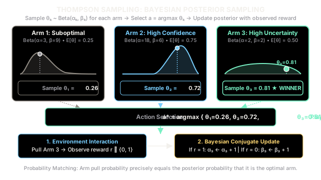
Thompson Sampling (also known as posterior sampling or probability matching) resolves this dilemma by formulating action selection within a Bayesian framework. Instead of maintaining single-point averages or artificial upper bounds, the agent maintains a full posterior probability distribution over the unknown parameters of each arm. In each round, it draws a sample from each posterior and greedily plays the arm that generated the highest draw.

Consequently, each action is selected with a probability exactly equal to the posterior probability that it is the optimal action:

$\mathbb{P}(A_t = a) = \mathbb{P}\left(\theta_a = \max_{a'} \theta_{a'} \mid \mathcal{H}_{t-1}\right)$

Arms with high epistemic uncertainty produce wide posterior distributions whose optimistic tails occasionally yield winning samples, driving natural exploration. As an arm is pulled and its uncertainty narrows, its posterior collapses around its true mean, smoothly transitioning the agent from exploration to exploitation without hand-crafted schedules.

Think of It Like This

How It Actually Works

Posterior Sampling and Beta-Bernoulli Conjugacy

Let $\mathcal{A} = \{1, 2, \dots, K\}$ denote a set of $K$ distinct actions (bandit arms). Each arm $k$ is characterized by an unknown true success probability $\theta_k^* \in [0, 1]$.

At each round $t = 1, 2, \dots, T$:

1. The agent selects an arm $a_t \in \mathcal{A}$.
2. The environment generates a binary reward $r_t \in \{0, 1\}$ from a Bernoulli likelihood:

$r_t \sim \text{Bernoulli}(\theta_{a_t}^*), \quad \mathbb{P}(r_t = 1 \mid \theta_{a_t}^*) = \theta_{a_t}^*$

To maintain Bayesian beliefs over each arm's parameter $\theta_k^*$, the agent places an independent Beta prior on each arm:

$\theta_k \sim \text{Beta}(\alpha_k, \beta_k)$

where $\alpha_k > 0$ represents prior pseudo-counts of successes, and $\beta_k > 0$ represents prior pseudo-counts of failures. An uninformative flat prior corresponds to $\alpha_k = 1$ and $\beta_k = 1$, which is equivalent to $\text{Uniform}(0, 1)$.

The Beta probability density function is:

$f(\theta; \alpha, \beta) = \frac{\theta^{\alpha - 1}(1 - \theta)^{\beta - 1}}{\mathrm{B}(\alpha, \beta)}, \quad \theta \in [0, 1]$

where $\mathrm{B}(\alpha, \beta) = \frac{\Gamma(\alpha)\Gamma(\beta)}{\Gamma(\alpha + \beta)}$ is the Beta function. The expected value and variance are:

$\mathbb{E}[\theta] = \frac{\alpha}{\alpha + \beta}, \quad \mathrm{Var}(\theta) = \frac{\alpha \beta}{(\alpha + \beta)^2(\alpha + \beta + 1)}$

The Thompson Sampling Decision Cycle:

1. Posterior Sampling: For each arm $k \in \{1, \dots, K\}$, draw an independent sample from its posterior distribution: $\hat{\theta}_k \sim \text{Beta}(\alpha_k, \beta_k)$
2. Action Selection: Select the arm with the highest sampled value: $a_t = \arg\max_{k \in \{1, \dots, K\}} \hat{\theta}_k$
3. Environment Feedback: Pull arm $a_t$ and observe reward $r_t \in \{0, 1\}$.
4. Bayesian Conjugate Update: Because the Beta distribution is conjugate to the Bernoulli likelihood, the posterior remains Beta. Update the parameters of the chosen arm $a_t$: $\alpha_{a_t} \leftarrow \alpha_{a_t} + r_t$ $\beta_{a_t} \leftarrow \beta_{a_t} + (1 - r_t)$ Unchosen arms ($k \neq a_t$) retain their previous parameter values.

Worked numerical example

Consider a 3-armed bandit problem ($K = 3$). At round $t = 1$, the agent holds the following beliefs:

• Arm 1 (Poor history): $\alpha_1 = 3, \beta_1 = 9 \implies \mathbb{E}[\theta_1] = \frac{3}{12} = 0.250$
• Arm 2 (High confidence, strong performance): $\alpha_2 = 18, \beta_2 = 6 \implies \mathbb{E}[\theta_2] = \frac{18}{24} = 0.750$
• Arm 3 (High uncertainty / underexplored): $\alpha_3 = 2, \beta_3 = 2 \implies \mathbb{E}[\theta_3] = \frac{2}{4} = 0.500$

Round 1:

• Step 1 (Sample): The agent draws random values from each arm's posterior:
  • $\hat{\theta}_1 \sim \text{Beta}(3, 9) \rightarrow 0.264$
  • $\hat{\theta}_2 \sim \text{Beta}(18, 6) \rightarrow 0.718$
  • $\hat{\theta}_3 \sim \text{Beta}(2, 2) \rightarrow 0.812$
• Step 2 (Select): $\arg\max \{0.264, 0.718, 0.812\} = \text{Arm 3}$. Even though Arm 2 has a substantially higher mean ($0.750 > 0.500$), Arm 3's high variance allows a draw from its optimistic upper tail, triggering exploration.
• Step 3 (Observe): The agent plays Arm 3 and receives reward $r_1 = 1$.
• Step 4 (Update):
  • $\alpha_3 \leftarrow 2 + 1 = 3$
  • $\beta_3 \leftarrow 2 + 0 = 2$
  • New mean: $\mathbb{E}[\theta_3] = \frac{3}{3 + 2} = 0.600$.

Round 2:

• Step 1 (Sample): The agent draws new samples:
  • $\hat{\theta}_1 \sim \text{Beta}(3, 9) \rightarrow 0.215$
  • $\hat{\theta}_2 \sim \text{Beta}(18, 6) \rightarrow 0.763$
  • $\hat{\theta}_3 \sim \text{Beta}(3, 2) \rightarrow 0.628$
• Step 2 (Select): $\arg\max \{0.215, 0.763, 0.628\} = \text{Arm 2}$. Arm 2 wins the draw, triggering exploitation of the proven leader.
• Step 3 (Observe): The agent plays Arm 2 and receives reward $r_2 = 1$.
• Step 4 (Update):
  • $\alpha_2 \leftarrow 18 + 1 = 19$
  • $\beta_2 \leftarrow 6 + 0 = 6$
  • New mean: $\mathbb{E}[\theta_2] = \frac{19}{19 + 6} = 0.760$.

Round 3:

• Step 1 (Sample): The agent draws new samples:
  • $\hat{\theta}_1 \sim \text{Beta}(3, 9) \rightarrow 0.312$
  • $\hat{\theta}_2 \sim \text{Beta}(19, 6) \rightarrow 0.735$
  • $\hat{\theta}_3 \sim \text{Beta}(3, 2) \rightarrow 0.540$
• Step 2 (Select): $\arg\max \{0.312, 0.735, 0.540\} = \text{Arm 2}$. Arm 2 wins again.
• Step 3 (Observe): The agent plays Arm 2 and receives reward $r_3 = 0$.
• Step 4 (Update):
  • $\alpha_2 \leftarrow 19 + 0 = 19$
  • $\beta_2 \leftarrow 6 + 1 = 7$
  • New mean: $\mathbb{E}[\theta_2] = \frac{19}{19 + 7} \approx 0.731$. The failure slightly decreases the mean and narrows the variance around $0.731$, fine-tuning future sampling draws.

Code

1import random2from typing import List3
4
5class BernoulliThompsonSampling:6    """Multi-armed bandit solver using Bayesian Bernoulli Thompson Sampling."""7
8    def __init__(self, n_arms: int, alpha_prior: float = 1.0, beta_prior: float = 1.0) -> None:9        self.n_arms = n_arms10        # Alpha tracks successes (+1 per success), Beta tracks failures (+1 per failure)11        self.alphas: List[float] = [alpha_prior] * n_arms12        self.betas: List[float] = [beta_prior] * n_arms13
14    def select_arm(self) -> int:15        """Draw one sample from each arm's posterior Beta distribution and pick the argmax."""16        samples = [17            random.betavariate(self.alphas[i], self.betas[i])18            for i in range(self.n_arms)19        ]20        return samples.index(max(samples))21
22    def update(self, arm: int, reward: int) -> None:23        """Update conjugate Beta posterior for the selected arm based on observed reward."""24        self.alphas[arm] += reward25        self.betas[arm] += (1 - reward)26
27    def expected_values(self) -> List[float]:28        """Return the posterior mean payoff probability for each arm."""29        return [30            self.alphas[i] / (self.alphas[i] + self.betas[i])31            for i in range(self.n_arms)32        ]33
34
35# Simulation: 3 arms with unknown true success probabilities36random.seed(42)37true_rates = [0.20, 0.75, 0.40]38bandit = BernoulliThompsonSampling(n_arms=len(true_rates))39
40pull_counts = [0] * len(true_rates)41total_reward = 042n_rounds = 100043
44for _ in range(n_rounds):45    arm = bandit.select_arm()46    reward = 1 if random.random() < true_rates[arm] else 047    bandit.update(arm, reward)48    pull_counts[arm] += 149    total_reward += reward50
51print(f"Pulls per arm: {pull_counts}")52print(f"Estimated means: {[round(m, 3) for m in bandit.expected_values()]}")53print(f"Total reward: {total_reward} / {n_rounds}")54
55# -> expected output:56# Pulls per arm: [10, 947, 43]57# Estimated means: [0.333, 0.751, 0.578]58# Total reward: 740 / 1000

Watch Out For

The Quick Version

• Probability Matching: Thompson Sampling selects each arm in direct proportion to the posterior probability that it is the optimal arm.
• Conjugate Mechanics: Under Bernoulli rewards, the Beta conjugate prior allows instant analytical updates ($\alpha \leftarrow \alpha + r$, $\beta \leftarrow \beta + (1 - r)$) without numerical integration or MCMC.
• Organic Exploration: High epistemic uncertainty naturally stretches the posterior distribution, generating optimistic tail samples that trigger exploration without manual $\varepsilon$-decay or bound tuning.
• Asymptotic Optimality: Achieves the theoretical lower bound on regret ($O(\log T)$ per the Lai-Robbins bound) while consistently outperforming heuristic alternatives in empirical benchmarks.

What to Read Next

• Multi-Armed Bandits
• Upper Confidence Bound (UCB)
• Epsilon-Greedy