LSTM for Forecasting

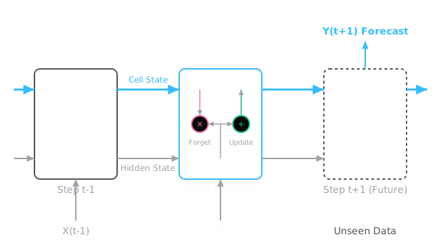
An LSTM carries a cell state across time steps, so a forecaster can remember last season while still reacting to this week.

Gates move the cell from 1.0 to 1.38 while the output gate reads out 0.62

Why Does This Exist?

A plain recurrent network reads a series step by step and multiplies its signal at every step, so after ten steps only a millionth of the first observation survives. A retailer forecasting December demand needs last December, not just last week, and that is exactly what plain recurrence drops first.

The LSTM fixes this with a second track, the cell state $C_t$ , which runs straight through time and is edited by addition instead of repeated multiplication. Gradients ride that additive path backward untouched, so old context survives the trip forward.

This page teaches the gated step: what each gate keeps, the one worked update, and where the forecast comes from. For the classical baseline that needs no gating, read SARIMA. When the horizon stretches past one step, the strategy question moves to multi-step forecasting.

Think of It Like This

The night-shift logbook with three highlighters

A warehouse runs a logbook that every shift inherits. The outgoing clerk carries three highlighters. First the grey one crosses out entries that no longer apply, like a discontinued product line. Then the green one copies only the important lines from tonight into the book. Finally the yellow one marks which lines the next clerk should read first.

The logbook is the cell state. The grey marker is the forget gate, the green one the input gate, the yellow one the output gate. Tonight's short summary passed at handover is the hidden state.

Where it stops: clerks understand what they cross out, while gates are learned weights with no notion of meaning. And a logbook never runs out of pages, while a fixed-size cell state must compress everything into one vector.

How It Actually Works

Call the current input $x_t$ , which means the observation at step $t$ . Call the short summary $h_t$ , which means the hidden state handed to the next step. Call the long book $C_t$ , which means the cell state carried forward. Each gate outputs numbers between 0 and 1, where 0 blocks everything and 1 lets everything through.

The forget gate decides what to erase, the input gate decides what to write, and the output gate decides what to read out. The cell update is pure addition, and that addition is the whole trick: nothing multiplies the carried value, so nothing shrinks it.

Worked example

Start with a cell of $C = 1.0$ . The forget gate opens at $f = 0.9$ , so $0.9 \times 1.0 = 0.9$ survives. The input gate opens at $i = 0.6$ on a candidate of $\tilde{C} = 0.8$ , so $0.6 \times 0.8 = 0.48$ gets added. The new cell is:

$C_{new} = 0.9 + 0.48 = 1.38$

Squash it with $\tanh$ , where $\tanh(1.38)$ is about $0.88$ . The output gate opens at $o = 0.7$ , so the hidden state handed on is $h = 0.7 \times 0.88 = 0.62$ . One number in, three gated moves, and the book moves from 1.0 to 1.38 while the next step sees only 0.62.

Code

This step function replays the worked example with nothing but the standard library:

1import math2
3
4def lstm_step(cell: float, forget: float, inp: float, cand: float, out: float) -> tuple[float, float]:5    new_cell = forget * cell + inp * cand6    hidden = out * math.tanh(new_cell)7    return round(new_cell, 2), round(hidden, 2)8
9
10print(lstm_step(1.0, 0.9, 0.6, 0.8, 0.7))  # -> (1.38, 0.62)

The printed pair matches the hand computation: the cell lands at 1.38 and the hidden state at 0.62. Change forget toward 0 and watch the first value collapse, which is the erasing behaviour the gate learns.

Watch Out For

Feeding unscaled prices into saturating gates

The symptom is a model that learns nothing while its gates sit at exactly 0 or 1. Raw inputs in the thousands push the sigmoid and $\tanh$ curves into their flat ends, where gradients vanish and weights freeze. Scale the series first, for example with min-max scaling fit on the training span only, and invert the scaling on the forecast. If gate activations histogram into spikes at the extremes, the inputs are too large.

Shuffling windows so the future leaks into training

The symptom is validation error far below live error. Building sliding windows before a chronological split lets windows from the same week land on both sides, and fitting a scaler on the full span smuggles test statistics into training. Split the timeline first, fit the scaler on the training span only, then build windows inside each span. If shuffling windows is needed, shuffle their order, never their contents.

The Quick Version

An LSTM adds a cell state to plain recurrence, so memory travels by addition instead of repeated multiplication.
The forget gate erases, the input gate writes, and the output gate reads, each with values between 0 and 1.
A cell of 1.0 with forget 0.9 and an addition of 0.48 lands at 1.38, and the output gate reads out 0.62.
The additive update is what keeps gradients alive across long gaps where plain recurrence keeps a millionth.
Scale inputs before they reach the gates and split the timeline before building windows.
Classical seasonality without gating lives in SARIMA, and horizons past one step belong to multi-step forecasting.