SARIMA

SARIMA reads last month for momentum and the same month last year for season, so July learns from June and from last July at once.

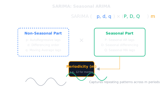
Why Does This Exist?

Plain ARIMA reads only the recent past, so it forecasts July from June and May while ignoring that July always spikes. Monthly airline passengers, December retail, and morning web traffic all repeat on a fixed calendar lag, and a model blind to that lag relearns the season from scratch every cycle.

SARIMA adds a seasonal twin of every ARIMA term operating $m$ steps back, where $m$ is the period: 12 for monthly data with a yearly cycle, 7 for daily data with a weekly cycle. The two halves multiply into one fit that reads June for momentum and last July for season together.

This page teaches the doubled order and its fixture. The non-seasonal parent it extends is ARIMA. The calendar-curve alternative that skips lags entirely is Prophet.

Think of It Like This

The returning festival vendor

A vendor returns to the same July festival each year. To stock this July she checks two things: how her June stall just did, because business momentum carries week to week, and how last July went, because the festival crowd dwarfs ordinary weeks. June alone would miss the festival entirely, while last July alone would miss that her business has grown since.

June is the non-seasonal half and last July the seasonal half. The period $m = 12$ is the twelve months between festivals. The multiplied fit is her stocking both signals at once.

Where it stops: vendors remember one festival, while SARIMA with a single $m$ learns exactly one cycle length. Two overlapping rhythms, such as daily and yearly, need richer models than one $m$ can state.

How It Actually Works

Write the order as $(p, d, q)(P, D, Q)_m$ . Call $p$ , $d$ , $q$ the short memory: past values, monthly differences, and past misses. Call $P$ , $D$ , $Q$ the same three ideas at seasonal distance: values, differences, and misses from $m$ , $2m$ , $3m$ steps back. Call $m$ the period, which means the fixed cycle length.

Seasonal differencing with $D = 1$ subtracts the value $m$ steps back, removing the repeating level so the short half works on surprises. The seasonal autoregression then weights last July directly, while the short autoregression weights June. Estimation fits all six orders jointly, not as two separate models.

Worked example

Take monthly passengers with $m = 12$ . Last July carried 150, June carried 160, and this July lands at 162. The seasonal difference is $162 - 150 = 12$ , which is the year-on-year growth with the festival effect removed. The monthly difference is $162 - 160 = 2$ , which is the short momentum into July. A SARIMA with $P = 1$ leans on the 150 from twelve steps back, while $p = 1$ leans on the 160 from one step back, and the fitted weights split the 162 between the two clues.

Code

This seasonal difference replays the fixture with only the standard library:

1def seasonal_diff(series: list[float], lag: int) -> list[float]:2    return [round(series[i] - series[i - lag], 2) for i in range(lag, len(series))]3
4
5past: list[float] = [140.0, 150.0, 142.0, 144.0, 146.0, 148.0, 150.0, 152.0, 154.0, 156.0, 158.0, 160.0, 160.0, 162.0]6print(seasonal_diff(past, 12)[-1])  # -> 12.07print(round(past[-1] - past[-2], 2))  # -> 2.0

The first output is the 12.0 year-on-year growth, and the second is the 2.0 monthly step. Raise the lag to 13 and the pairing breaks, which is exactly what a wrong $m$ does to the seasonal half.

Watch Out For

Differencing twice until only noise remains

The symptom is a variance that grows after differencing and a lag-1 autocorrelation that flips negative. With $d = 1$ and $D = 1$ the series is differenced twice, which overdoses a series whose season was already mild. Difference once, check stationarity, and stop: if the seasonal difference alone flattens the level, leave $d$ at 0. A variance that rises instead of falls is the signal to back off.

Setting m to 365 on daily data with yearly season

The symptom is a fit that never finishes or demands decades of history for a handful of seasonal weights. A period of 365 turns every seasonal term into a year-long reach with sparse evidence per lag. Prefer Fourier terms or a calendar model such as Prophet for long periods, and reserve SARIMA for short single cycles like $m = 7$ or $m = 12$ .

The Quick Version

SARIMA multiplies a short-memory $(p, d, q)$ half by a seasonal $(P, D, Q)$ half at period $m$ .
The period $m$ is the fixed cycle length: 12 for monthly data with a yearly season, 7 for daily data with a weekly one.
Seasonal differencing subtracts the value $m$ steps back, so 162 minus last July 150 leaves growth of 12.
The short half reads June at 160 for momentum while the seasonal half reads last July at 150 for the festival.
One $m$ learns one rhythm, so overlapping daily and yearly cycles need a different model.
ARIMA is the non-seasonal parent, and Prophet is the curve-fitting alternative without lags.