Probabilistic Forecasting

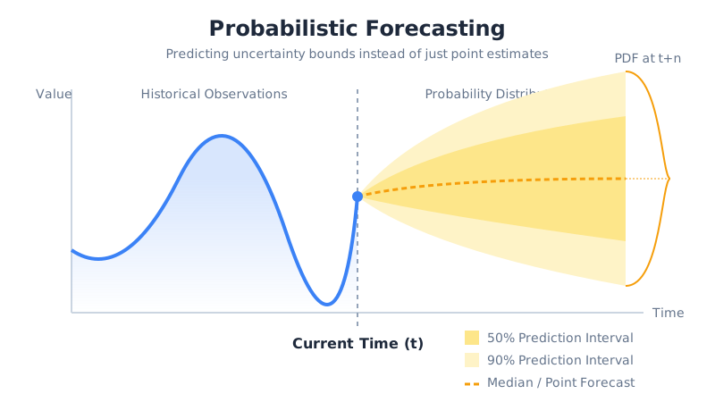
A point says demand will be 100, while a band says 92 to 108 with 90 percent confidence, and only the band tells you how much safety stock to hold.

A point forecast is one line while the 10th to 90th band widens with each step ahead

Why Does This Exist?

A point forecast of 100 units next week is always wrong, and the one number never says by how much. When a stockout costs ten times an overstock, the median is the wrong order quantity: the business wants the 90th percentile, not the middle.

Probabilistic forecasting replaces the single number with a distribution per step, usually reported as quantiles or intervals. A 90 percent band of 92 to 108 means the planner can price the risk instead of guessing it.

This page teaches quantiles, the loss that trains them, and the coverage check that keeps them honest. The horizon they widen across is multi-step forecasting, and a business model that already ships bands is Prophet.

Think of It Like This

The river guide calling the crossing window

A guide never promises the river will be exactly waist-deep at noon. She says it runs knee to chest on nine mornings out of ten, and picks the crossing hour from the shallow edge of that window. The single depth number would send the group in blind, while the window tells them when to go and what to wear.

The window edges are the 10th and 90th quantiles. The nine mornings out of ten are empirical coverage. The shallow-edge choice is ordering at a high quantile because a soaking costs more than a wait.

Where it stops: rivers answer to weather the guide can see, while demand answers to shocks no model observes. The band quantifies the usual wobble, never the once-a-decade flood.

How It Actually Works

Call the quantile level $\tau$ , which means the share of outcomes that should fall at or below the forecast. The median is $\tau = 0.5$ . The band edges in the diagram are $\tau = 0.1$ with value 92 and $\tau = 0.9$ with value 108 around a median of 100.

Quantiles train on the pinball loss, which punishes each side asymmetrically. For actual $y$ and forecast $\hat{y}$ at level $\tau$ with error $e = y - \hat{y}$ , the loss is $\max(\tau e, (\tau - 1) e)$ . At $\tau = 0.9$ an underestimate of 5 costs $0.9 \times 5 = 4.5$ while an overestimate of 5 costs only $0.1 \times 5 = 0.5$ , so the 90th percentile learns to sit high.

Worked example

Fix actual demand $y = 100$ . A 90th-percentile forecast of 95 misses low by 5, and the loss is $\max(0.9 \times 5, -0.1 \times 5) = \max(4.5, -0.5) = 4.5$ . A 10th-percentile forecast of 105 misses high by 5, and the loss is $\max(0.1 \times -5, -0.9 \times -5) = \max(-0.5, 4.5) = 4.5$ . Both misses cost 4.5 because each quantile fears its own dangerous side.

Then check honesty: run 100 past weeks through the 90 percent band and count. If 90 land inside, the band is calibrated. If only 70 land inside, the model is overconfident no matter how small its loss looked.

Code

This pinball function replays both sides of the worked example:

1def pinball(actual: float, forecast: float, level: float) -> float:2    error = actual - forecast3    return round(max(level * error, (level - 1.0) * error), 2)4
5
6print(pinball(100.0, 95.0, 0.9))  # -> 4.57print(pinball(100.0, 105.0, 0.1))  # -> 4.5

Both calls print 4.5, confirming the asymmetry: the high quantile is punished for sitting low, the low quantile for sitting high, and each learns its own edge of the band.

Watch Out For

Quoting bands that never passed a coverage count

The symptom is a crisp 90 percent band that reality escapes far more than one week in ten. Uncalibrated intervals read as promises while behaving as guesses. Count empirical coverage on a held-out span before quoting any band: 90 of 100 inside for a 90 percent claim. If the count is 70, widen the band or recalibrate instead of shipping the number.

Forcing symmetric bands onto one-sided risk

The symptom is a Gaussian interval that dips below zero demand or misses the long upside tail. Real constraints bite on one side: stock cannot go negative, while spikes run tenfold up. A symmetric $\mu \pm 2\sigma$ band wastes half its width where nothing can happen. Prefer direct quantiles, which let 92 and 108 sit at uneven distances from 100.

The Quick Version

Probabilistic forecasting outputs quantiles and intervals per step instead of one point per step.
The pinball loss punishes each side by its level, so a miss of 5 costs 4.5 at both the 90th and 10th edges.
A median of 100 with a 90 percent band of 92 to 108 turns safety stock into arithmetic.
Bands widen with horizon, which is why the horizon plan in multi-step forecasting comes first.
Count coverage on held-out weeks: 90 of 100 inside means the 90 percent band is honest.
Asymmetric risk needs quantiles, never a forced symmetric bell.